Emerging Markets Macro Factor Model: A Data Science Approach to Global Finance
Emerging markets sit at the intersection of global and local forces. They are exposed to shifts in U.S. rates, dollar strength, volatility, and commodities, but they are also shaped by country-specific regulation, politics, sector mix, and domestic demand. That makes a basic question surprisingly hard to answer: how much of EM equity performance is really global macro, and how much is local noise?
This project tackles that question with a PCA-based macro factor model built on ten years of daily data. Using Bloomberg-sourced MSCI country indices and a focused set of global macro series, I compress correlated macro variables into a few orthogonal factors, regress country equity returns on those factors, and then track the model’s explanatory power through time with rolling-window analysis.
The result is a framework that is useful in two ways. First, it gives a cleaner cross-sectional view of which markets are structurally more macro-sensitive. Second, it shows that macro sensitivity is highly regime-dependent: modest in calm periods, but much more powerful during global stress episodes such as COVID, tariff shocks, and tightening cycles.
What is an Equity Factor Model?
An equity factor model is a toolkit for explaining returns using systematic drivers. Instead of treating market moves as random, the model attributes performance to quantifiable forces like currencies, interest rates, commodities, or volatility. For investors, this makes abstract market movements more tangible:
- Risk attribution: Which macro factors matter most right now?
- Portfolio construction: How should EM weights shift with the macro cycle?
- Risk management: Where are exposures hiding that could amplify a shock?
- Market timing: How do sensitivities evolve through different regimes?
In short, a factor model is about turning noisy markets into interpretable signals, bridging raw data and actionable investment insight.
Executive Summary
Using ten years of daily data for Brazil, Mexico, South Africa, China, India, Indonesia, Taiwan, Korea, and the United States, I extract global macro factors via Principal Component Analysis and then regress country equity returns on those factors.
Three high-level results stand out:
- Global macro factors explain a meaningful but modest share of daily EM return variation in the full sample.
- The first three principal components capture about 65% of total macro variance, and adding more components only marginally improves average model fit.
- Macro influence is episodic rather than constant. It spikes sharply during stress periods such as the China growth scare, the tariff cycle, COVID, and aggressive U.S. tightening.
Across the full sample, Brazil and Mexico emerge as the most macro-sensitive markets, while China, India, Taiwan, and Indonesia are less consistently explained by the global factor set. The broader message is that EM equities are not permanently “macro trades,” but they can become highly macro-driven when global risk premia compress into a single market regime.
Data Universe
Equity Markets
The equity side of the model uses daily MSCI country index levels for:
- Brazil
- Mexico
- South Africa
- China
- India
- Indonesia
- Taiwan
- Korea
- United States as a benchmark
Global Macro Variables
The final implemented macro factor set uses seven variables:
- USD Index (DXY) for dollar strength
- Brent crude for commodity and energy sensitivity
- U.S. 10Y yield for long-duration discount rates
- U.S. 2Y yield for policy sensitivity
- VIX for global risk aversion
- BAA credit spread for corporate risk premium conditions
- U.S. term spread for curve shape and recession signaling
These variables are intentionally overlapping. That is exactly why PCA is useful here: it compresses them into orthogonal latent factors that are easier to interpret and less vulnerable to multicollinearity.
Workflow
1. Data Collection
The data pipeline was built in Bloomberg BQuant using BQL. The raw index levels and macro series were pulled at daily frequency and then exported into a combined dataset for analysis.
2. Log Returns and Term-Spread Engineering
Before running PCA, all series are converted into daily log returns to make the inputs more stationary and scale-consistent. One nuance is the term spread: because it can go negative, it cannot always be log-transformed directly. To handle that, the series is shifted only when necessary before computing log returns.
shift_value = df['Term_Spread'].min()
if shift_value < 0.0:
    shift_value = df['Term_Spread'].min() - 0.1
else:
    shift_value = 0.0

df['Term_Spread_Engineered'] = df['Term_Spread'] - shift_value
df.drop(columns=['Term_Spread'], inplace=True)
df.rename(columns={'Term_Spread_Engineered': 'Term_Spread'}, inplace=True)

log_returns = np.log(df / df.shift(1)).dropna()
In the sample used here, the adjustment ended up not being needed because the minimum term spread stayed positive, but the transformation logic matters for robustness across regimes.
3. Separate Equity Returns from Macro Returns
The model treats EM country returns as dependent variables and macro returns as PCA inputs:
Y = log_returns[em_columns]
X = log_returns[macro_columns]
In the final dataset:
Yhas shape(3652, 9)Xhas shape(3652, 7)
4. Standardize Macro Inputs
Because PCA is variance-sensitive, the macro matrix is standardized first:
scaler = StandardScaler()
X_scaled = scaler.fit_transform(X)
5. Run PCA via SVD
Rather than treating PCA as a black box, this workflow computes it explicitly with singular value decomposition:
U, S, Vt = np.linalg.svd(X_scaled, full_matrices=False)
loadings = Vt.T
scores = U @ np.diag(S)
eigenvalues = (S ** 2) / (n_samples - 1)
exp_ratio = eigenvalues / eigenvalues.sum()
This makes the geometry clearer:
loadingstell us which macro variables define each componentscoresare the component time series used in regressionsexp_ratiotells us how much variance each component captures
Choosing the Number of Principal Components
To determine how many macro components are actually useful, I compare the average regression R² across markets with the cumulative variance explained by the first n PCs.
| PCs | Avg R² | Variance Captured |
|---|---|---|
| 1 | 0.079 | 31.5% |
| 2 | 0.158 | 49.8% |
| 3 | 0.164 | 65.0% |
| 4 | 0.165 | 76.7% |
| 5 | 0.175 | 87.6% |
| 6 | 0.180 | 96.8% |
| 7 | 0.181 | 100.0% |
This is the cleanest model-selection result in the project. The jump from one to two PCs matters. The jump from two to three still helps. After that, the marginal gain in average explanatory power is small. That makes three PCs a sensible compromise between interpretability and performance.
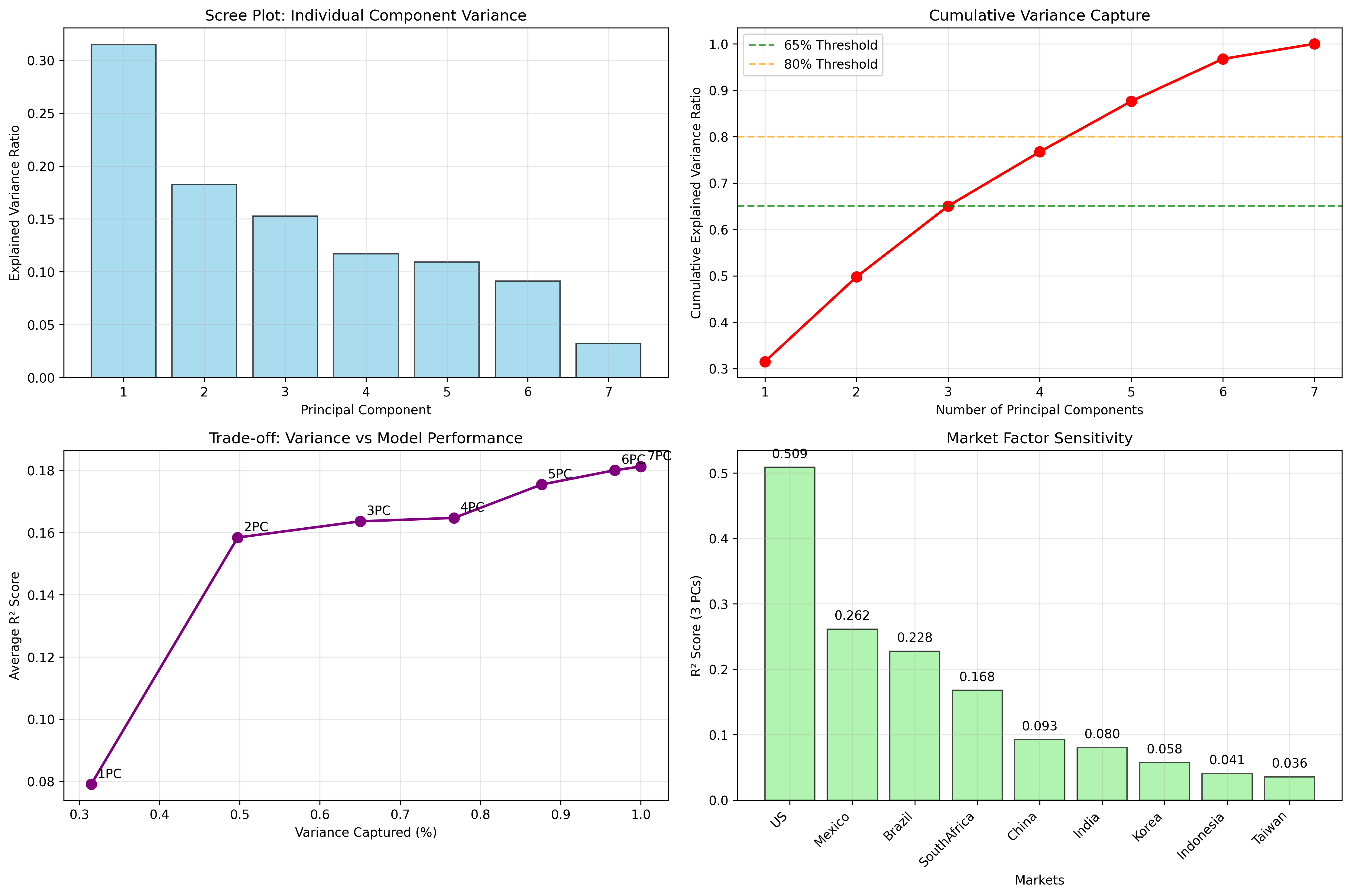
Figure: Variance captured by successive principal components and the trade-off against average model fit. Three components preserve most of the signal without making the model much harder to interpret.
Interpreting the Top 3 Macro Factors
PC1: Rates and Broad Financing Conditions
Top absolute loadings:
- U.S. 10Y yield:
0.578 - U.S. 2Y yield:
0.534 - BAA spread:
0.388 - VIX:
0.322 - Brent oil:
0.318
PC1 is best understood as a rates-and-risk-premium factor. It moves with Treasury yields, credit conditions, and volatility, so it captures shifts in discount rates and global financing conditions.
PC2: Dollar and Risk Sentiment
Top absolute loadings:
- USD Index:
0.637 - VIX:
0.418 - BAA spread:
0.378 - Brent oil:
0.337 - U.S. 2Y yield:
0.333
PC2 behaves like a risk-on / risk-off factor, centered on the dollar, volatility, and commodity pressure. This is the classic macro regime investors often associate with EM performance.
PC3: Yield-Curve Signal
Top absolute loadings:
- Term spread:
0.912 - VIX:
0.281 - U.S. 10Y yield:
0.213 - USD Index:
0.186 - BAA spread:
0.091
PC3 is overwhelmingly a yield-curve and cycle-expectations factor. It is the cleanest of the three components conceptually, because the term spread dominates the loading structure.
Which Markets Are Most Macro-Sensitive?
Using the three-factor specification, I regress each market’s daily returns on PC1 through PC3 and compare fit across countries. The pattern is intuitive:
- Brazil and Mexico have the highest macro sensitivity
- China, India, Taiwan, and Indonesia are less consistently explained by the global factor set
- The United States, included as a benchmark, also shows meaningful macro sensitivity
That cross-section lines up with market structure. Brazil and Mexico are more exposed to commodities, external financing conditions, and global risk appetite. Several Asian markets, by contrast, retain stronger domestic-policy and sector-specific drivers that dilute pure macro transmission.
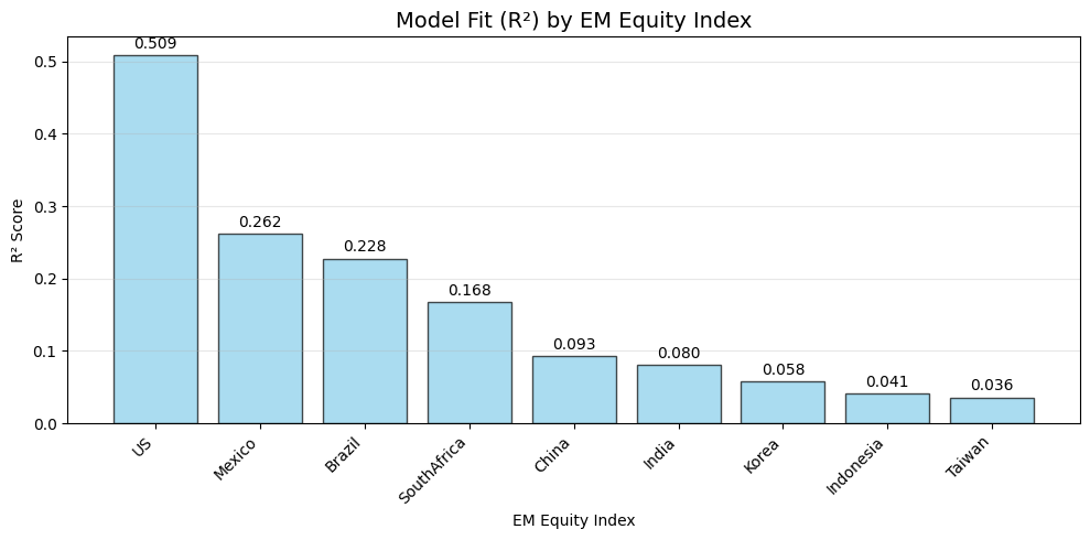
Figure: Full-sample model fit by market. Higher R² means a larger share of that market’s daily return variation is explained by the macro factor model.
Regime Shifts Across Recent Periods
The full-sample results are useful, but the story changes across regimes. The model behaved differently during post-COVID reopening, the global tightening cycle, and the more recent normalization period:
- 2022/2023: reopening and inflation pressure kept macro sensitivity elevated
- 2023/2024: aggressive tightening and policy divergence created more differentiated country responses
- 2024/2025: markets began settling into a new equilibrium, with selective decoupling across EMs
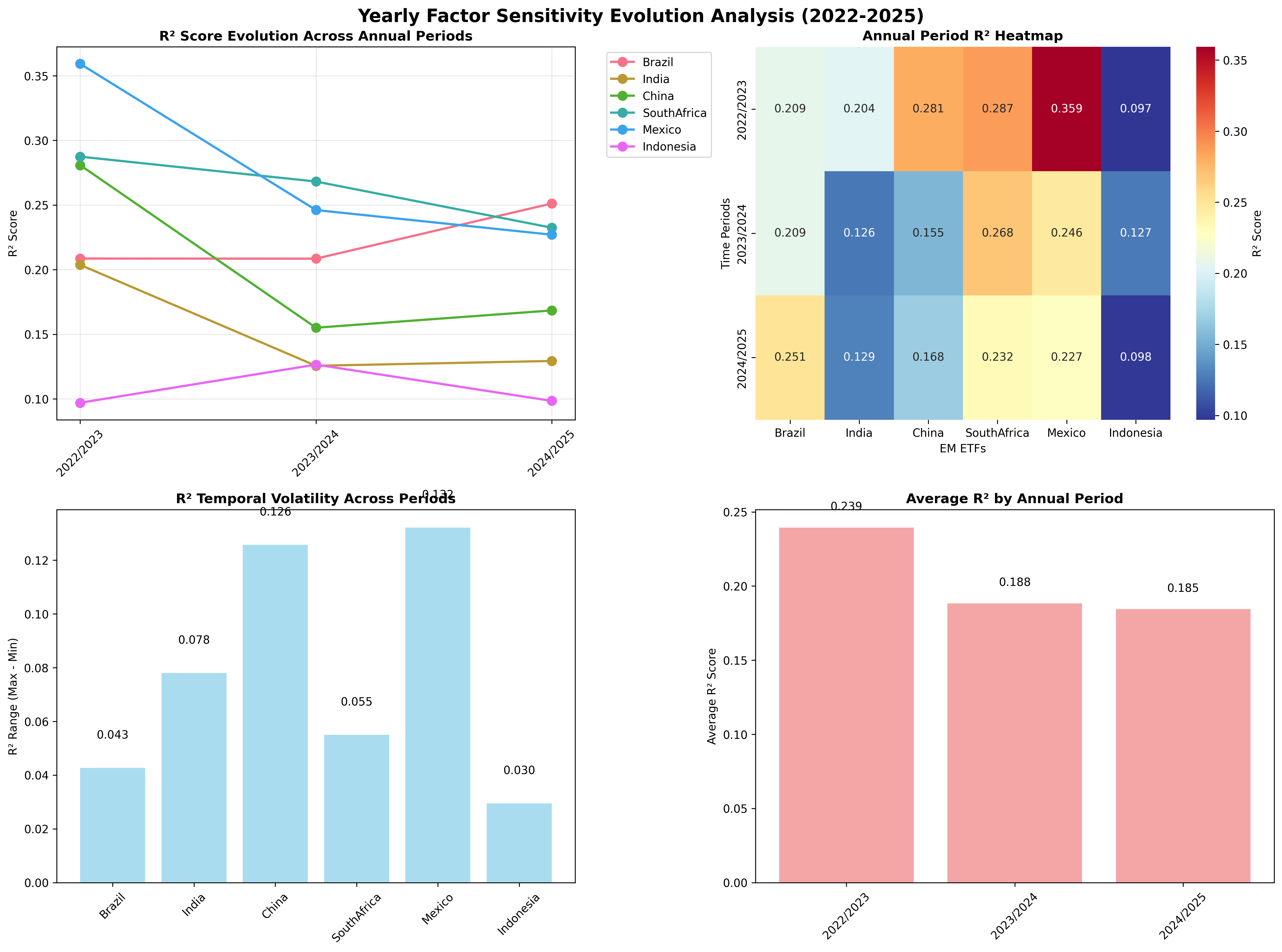
Figure: Evolution of factor sensitivity across recent periods, showing that macro integration is not static and can shift meaningfully from one regime to the next.
Rolling Regression Analysis
The static regression is useful, but the rolling analysis is where the model becomes much more interesting.
Using a 60-day rolling window, I recompute PCA and re-estimate the factor model through time:
def rolling_r2_scores_svd(X, Y, window=60, n_components=3):
    results = pd.DataFrame(index=Y.index[window:], columns=Y.columns, dtype=float)

    for i in range(window, len(Y)):
        X_win = X.iloc[i - window:i]
        Y_win = Y.iloc[i - window:i]

        X_scaled = StandardScaler().fit_transform(X_win)
        U, S, Vt = np.linalg.svd(X_scaled, full_matrices=False)
        scores_window = U[:, :n_components] @ np.diag(S[:n_components])

        for col in Y.columns:
            results.at[Y.index[i], col] = LinearRegression().fit(
                scores_window, Y_win[col].values
            ).score(scores_window, Y_win[col].values)

    return results
This produces a time series of rolling R² values for each market, showing when global macro factors become more or less dominant.
What the Rolling Results Show
The time variation is the core insight of the project:
- In calm periods, macro factors usually explain only a modest share of daily return variation
- During stress episodes, the explanatory power of macro factors rises sharply
- COVID produced the most dramatic synchronization, with rolling
R²values for some markets briefly pushing into the 0.6 to 0.8 range - China also showed a secondary jump around the late trade-war / post-trade-war period, suggesting that geopolitical shocks can temporarily increase macro transmission
This is why I think the model is more useful as a regime detector than as a constant forecasting tool. It helps identify when EM markets are trading like macro assets rather than simply assuming they always do.
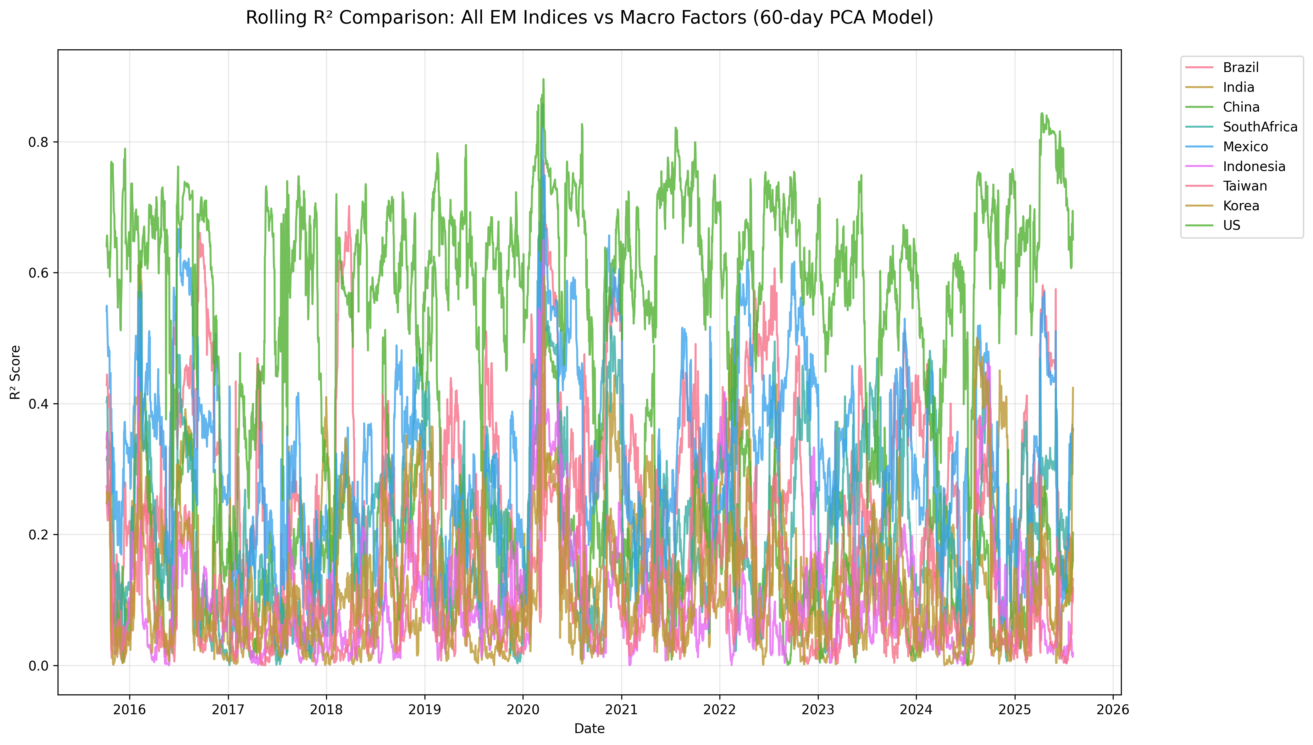
Figure: Rolling R² comparison across markets using a 60-day window. Crisis periods create obvious spikes in macro co-movement, while calmer periods show much weaker common-factor influence.
Representative Market Snapshots
The aggregate chart is useful, but a few single-country views make the pattern easier to see:
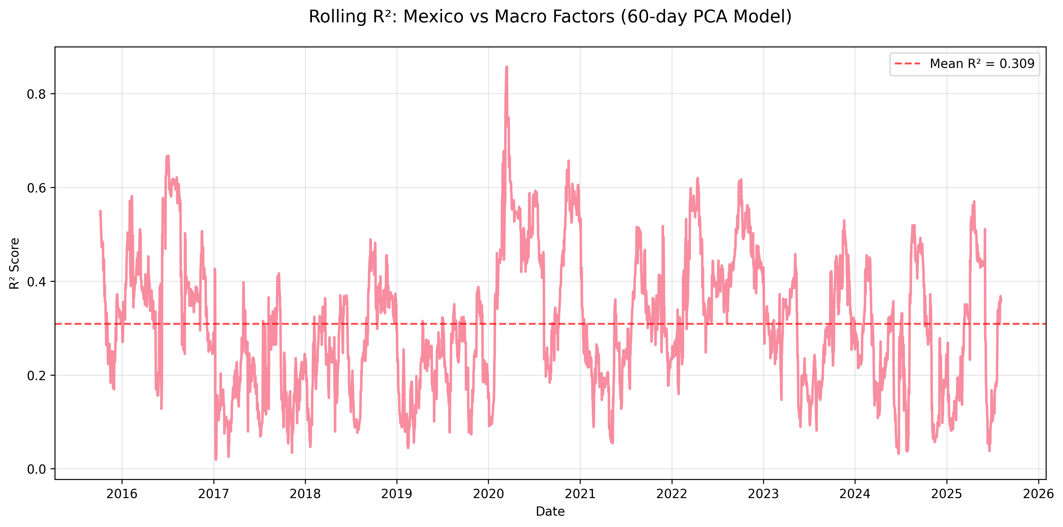
Figure: Mexico’s rolling R² shows one of the clearest and most persistent macro linkages in the sample, consistent with external trade exposure and sensitivity to global risk conditions.
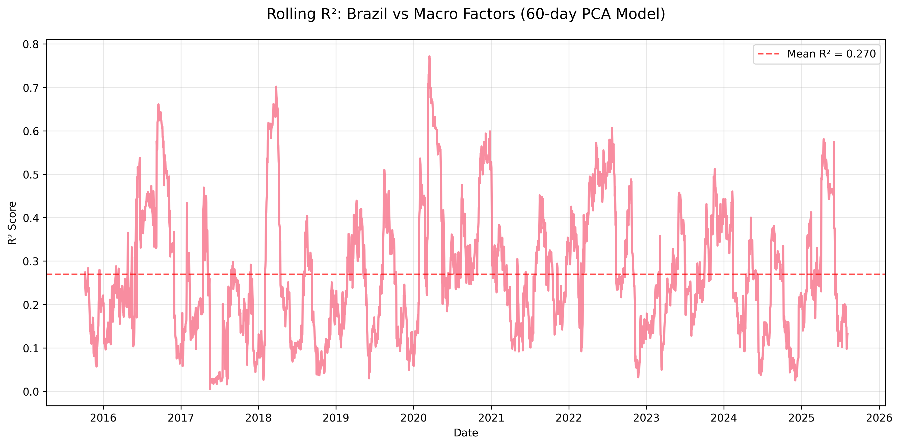
Figure: Brazil also shows meaningful macro sensitivity, but with more regime variation, reflecting a mix of commodity exposure and domestic political or policy noise.
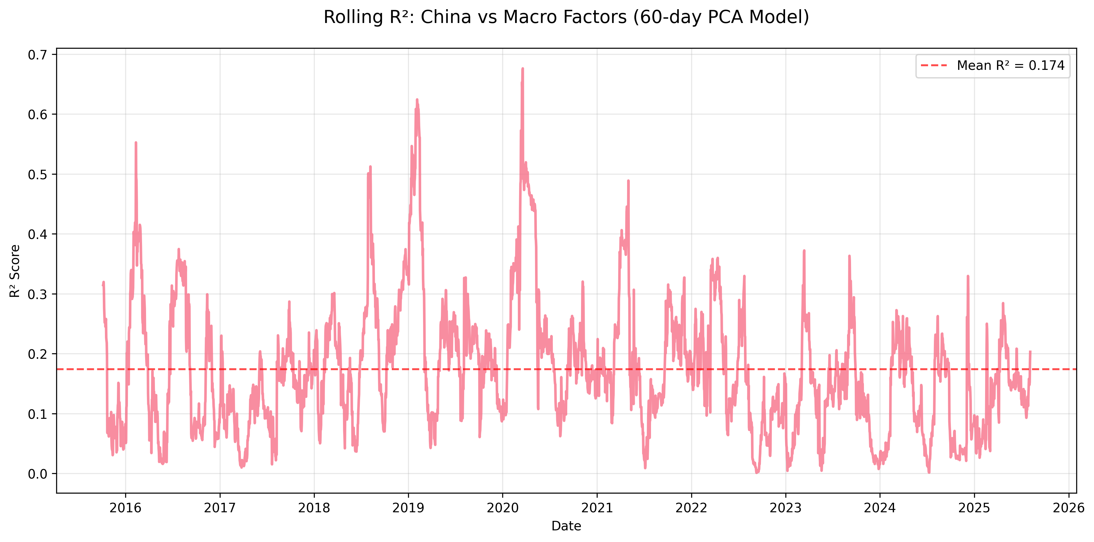
Figure: China’s rolling R² is lower on average, but still exhibits distinct spikes during major global or geopolitical stress episodes, which is exactly the kind of episodic transmission this framework is meant to detect.
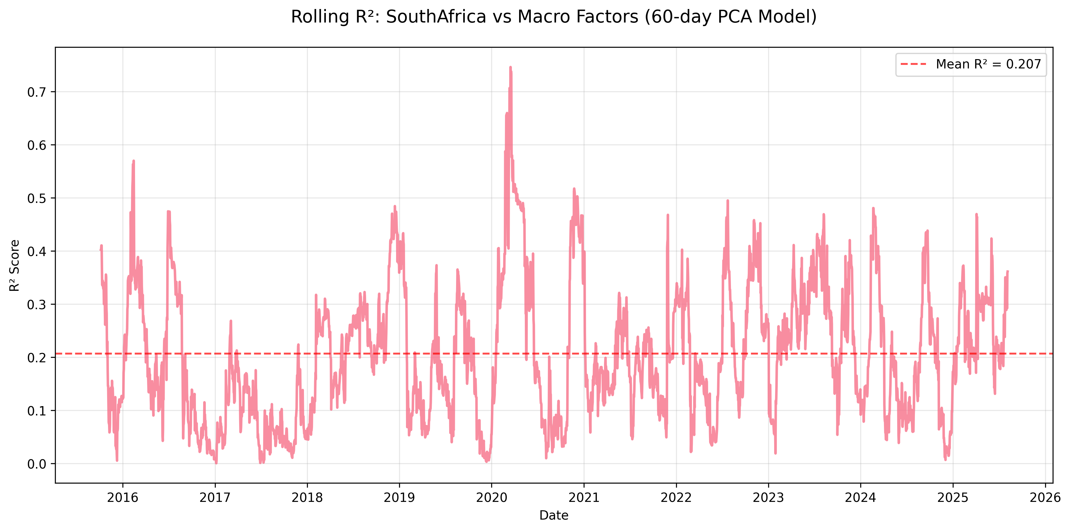
Figure: South Africa sits in the middle of the spectrum, with visible macro sensitivity but less consistency than Mexico, underscoring how capital flows and commodity exposure can amplify regime dependence without fully dominating the market.
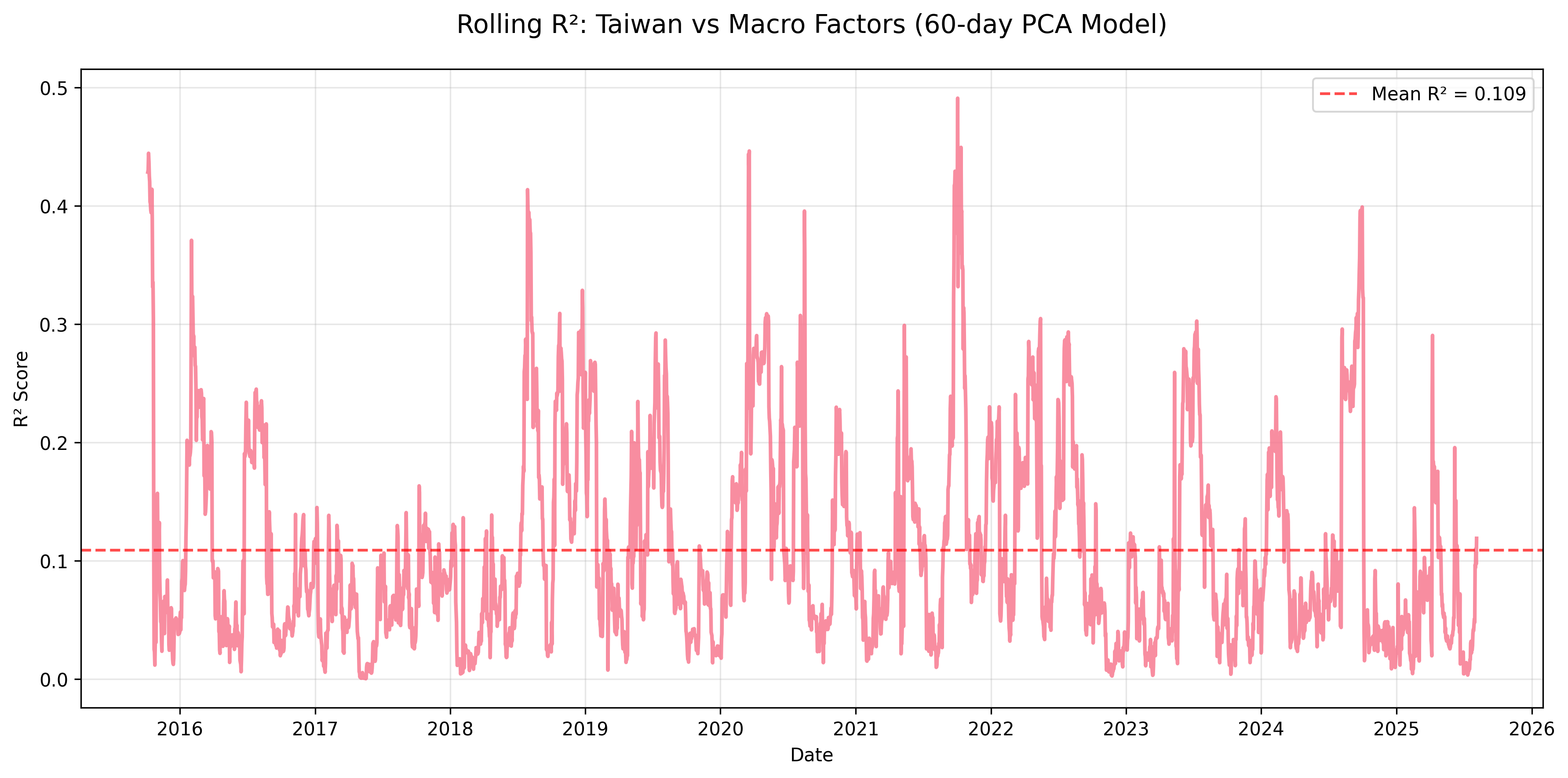
Figure: Taiwan provides the clearest contrast case. Its rolling R² is generally much lower, which reinforces the point that some EM markets remain much more sector- and locally driven outside of global stress windows.
Why This Matters
This framework is helpful for several practical questions:
- Risk budgeting: which EM positions are likely to behave like macro trades?
- Portfolio construction: where do you really have diversification versus disguised global beta?
- Stress testing: how much should you expect cross-market correlations to rise in crisis conditions?
- Narrative discipline: when performance is weak, is the driver local execution or global macro compression?
That last point matters. EM investing often gets reduced to storytelling, but a structured macro model can show when those stories matter less than global rates, dollar strength, or volatility.
Conclusion
The best summary is simple: global macro factors matter for EM returns, but not all the time, and not equally across countries.
Across the full sample, the model explains a moderate share of daily return variation. Three principal components are enough to capture most of the relevant macro structure. Brazil and Mexico are the most globally sensitive markets in the sample. China, India, Taiwan, and Indonesia are less consistently explained by the common macro factor set. And during major risk-off episodes, macro influence rises dramatically as cross-market behavior converges.
That combination of cross-sectional and time-varying insight is what makes the approach useful. It does not claim that EM returns are “just macro.” Instead, it shows that EM markets oscillate between locally driven and globally synchronized regimes, and that those regime shifts are measurable.
Next Steps
There are several natural extensions to this work:
- include additional macro variables such as liquidity or sovereign spreads
- compare daily, weekly, and monthly horizons
- test sector-level EM indices rather than country aggregates
- replace static linear regressions with regime-switching or state-dependent models
But even in its current form, the model provides a solid bridge between quantitative rigor and market intuition: it turns a messy global macro backdrop into a smaller, interpretable set of factors and shows when those factors really matter.
Data, Code, and Visuals
The companion project materials are grouped below for easier navigation.
Data and Repository
Notebooks
- Data acquisition notebook
- Factor modeling notebook
- Visualization and analysis notebook
- Summary report notebook