Emerging Markets Macro Factor Model: A Data Science Approach to Global Finance
Emerging Markets Macro Factor Model: A Data Science Approach to Global Finance
Emerging markets often sit at the crossroads of global and local forces. On one hand, they are deeply exposed to shifts in global liquidity, U.S. interest rates, dollar strength, and commodity cycles. On the other hand, their returns are just as often driven by uniquely domestic dynamics — policy choices, industrial structures, or country-specific shocks. This duality makes them fascinating but also notoriously difficult to model: are EM equities primarily a reflection of global macro tides, or do they chart their own course?
That question is at the heart of this project. We set out to build a multi-factor equity model that could disentangle the relative weight of global versus local drivers in EM performance. Using Bloomberg’s BQuant platform, we combined Principal Component Analysis (PCA) to compress complex macro datasets into interpretable factors, rolling regressions to track how relationships evolve through time, and visual analytics to highlight patterns that static models often miss. The result is a framework that bridges quantitative rigor with intuitive storytelling — one that lets us say not just how much EM markets are explained by global macro, but also when and why.
This matters for investors because EM sensitivity is rarely constant. During normal times, local dynamics dominate and global factors explain only a modest share of returns. But during periods of stress — think the 2015/16 China growth scare, tariff threats in 2018, COVID-19, or Fed tightening cycles — global forces can suddenly explain the bulk of the variance, sweeping diverse markets into the same tide. Understanding this ebb and flow is critical for risk management, portfolio construction, and alpha generation.
In the sections that follow, we’ll first define what a factor model is and why it’s useful, then walk through the design of our EM macro model, and finally highlight key results. Along the way, we’ll explore not just the top three principal components, but also secondary factors, specific crisis periods, and rolling-window dynamics. The goal is to provide a nuanced but approachable view of how global and local forces shape emerging market equities.
What is an Equity Factor Model?
An equity factor model is a toolkit for explaining returns using systematic drivers. Instead of treating market moves as random, the model attributes performance to quantifiable forces like currencies, interest rates, commodities, or volatility. For investors, this makes abstract market movements more tangible:
- Risk attribution: Which macro factors matter most right now?
- Portfolio construction: How should EM weights shift with the macro cycle?
- Risk management: Where are exposures hiding that could amplify a shock?
- Market timing: How do sensitivities evolve through different regimes?
In short, a factor model is about turning noisy markets into interpretable signals — bridging raw data and actionable investment insight.
🌍 Executive Summary
This project set out to answer a simple but important question: how much of emerging market equity performance is explained by global macro forces versus local dynamics? Using Bloomberg’s BQL platform, we built a macro factor model that connects EM index returns to drivers like the dollar, interest rates, volatility, and commodities. The analysis combines several complementary angles:
- Principal Components Analysis (PCA): distilling global macro variables into a small set of common risk factors.
- Extended factor exploration: examining not only the top three PCs but also lower-order components that capture subtler themes.
- Time dynamics: testing the model over specific historical windows and through rolling regressions to see how macro sensitivity evolves.
The results show a clear pattern: most EMs are not strongly explained by global macro factors under normal conditions. Instead, local policy choices, sectoral mix, and country-specific events dominate. But during crisis episodes global macro factors surge in importance, temporarily driving much larger shares of EM return variance.
At the cross-section level, we find meaningful differences across countries. Mexico and Brazil stand out as the most macro-sensitive markets, reflecting trade ties, commodity exposures, and capital flow dependence. Taiwan, Korea, and India sit at the other extreme, with returns largely shaped by local drivers such as tech cycles, industrial policy, or domestic demand. China, while globally significant, also shows surprisingly low macro sensitivity, underlining the importance of its policy-driven market structure.
For practitioners, this framework offers more than just an academic exercise. It highlights where EM exposures are likely to behave like leveraged plays on global risk, and where diversification potential lies in markets driven by local dynamics. Looking ahead, the model could be extended by incorporating additional factors (credit spreads, liquidity indicators, geopolitical risk indices), testing alternative horizons, and comparing sensitivity across asset classes.
In short: emerging markets are not monolithic. They oscillate between being swept up by global tides and charting their own course. This analysis helps investors understand when — and where — each force is likely to dominate.
Project Overview: Comprehensive Factor Analysis 🚀
Our implementation uses a multi-step approach with several key features for better insight:
1. Data Universe & Methodology 📊
Emerging Market Country Indices (MSCI):
- Brazil: Latin America’s largest economy, commodity-driven
- India: South Asian technology and services hub
- China: World’s second-largest economy, manufacturing powerhouse
- South Africa: African markets gateway, mining & resources
- Mexico: NAFTA/USMCA integration, manufacturing hub
- Indonesia: Southeast Asian commodity exporter
- Taiwan: Technology manufacturing capital
- Korea: Advanced EM market, export-oriented economy
- US: Developed market benchmark for comparison
Macro Factors:
- USD Index (DXY): Dollar strength vs. major currencies
- Oil (Brent): Global energy prices and commodity cycles
- US 10Y Yield: Risk-free rate benchmark and capital flows
- US 2Y Yield: Fed policy proxy, affects carry trades
- VIX: Market volatility and risk sentiment
- Credit Spreads (BAA): Corporate risk premium indicator
- Term Spread: Yield curve slope (10Y - 2Y), growth expectations
2. Analytical Framework ⚡
Principal Component Analysis (PCA)
Instead of using raw macro factors (which suffer from multicollinearity), we apply PCA to:
- Reduce dimensionality from 7 enhanced factors to 3 principal components
- Capture 65% of macro factor variance
- Eliminate multicollinearity issues
- Create orthogonal factors for cleaner interpretation
Multi-Factor Regression Model
EM Index Return = α + β₁×PC1 + β₂×PC2 + β₃×PC3 + ε
Rolling Window Analysis
- 60-day rolling windows for time-varying analysis
- Dynamic R² tracking to monitor model stability
- Regime identification through changing factor sensitivity
3. Technical Implementation Overview
| Component | Method | Purpose |
|---|---|---|
| Data Source | Bloomberg BQL API | Real-time market data |
| Asset Universe | MSCI EM indices + enhanced macro factors | Institutional-grade benchmarks |
| Preprocessing | Log returns transformation | Stationarity for modeling |
| Dimensionality Reduction | PCA with standardization | Orthogonal factor extraction |
| Model Estimation | Linear regression | Factor loading estimation |
| Validation | Rolling analysis + hand chosen windows | Time-varying performance |
Data Acquisition & Processing 📥
We use Bloomberg’s BQL within the BQuant environment to access both index and macroeconomic data, which we then save into a CSV file for efficient reloading.
- Time Period: 10-year lookback for statistical robustness and long-term factor stability
- Missing Data: Bloomberg’s native forward-fill methodology for market holidays
# =============================================================================
# STEP 0: LOAD ESSENTIAL LIBRARIES
# =============================================================================
#Core data manipulation
import pandas as pd
import numpy as np
import os
# =============================================================================
# STEP 1: Create helper function for extracting date for multiple time series
# =============================================================================
def fetch_bql_series(assets, bql_service, date_range):
    """
    Fetches time series data for given assets using Bloomberg Query Language (BQL).

    This function provides a streamlined interface to Bloomberg's data,
    handling multiple asset queries efficiently and returning clean pandas DataFrames.

    Parameters:
    -----------
    assets : dict
        Dictionary mapping asset names to Bloomberg tickers
        Example: {'Brazil': 'MXBR Index', 'USD_Index': 'DXY Curncy'}
    bql_service : bql.Service
        Authenticated Bloomberg Query Language service instance
    date_range : bql.func.range
        Bloomberg date range object (e.g., bq.func.range('-10Y', '0D'))

    Returns:
    --------
    pd.DataFrame
        DataFrame with datetime index and columns for each asset
        All data is automatically forward-filled by Bloomberg for quality

    Notes:
    ------
    - Uses PX_LAST field for consistent daily closing values
    - Bloomberg handles missing values with native forward-fill
    """
    data = {}

    # Iterate through each asset and fetch time series
    for asset_name, ticker in assets.items():
        # Execute BQL query for last price over specified date range
        query = bql_service.time_series(ticker, "PX_LAST", date_range[0], date_range[1])

        # Extract value column and store with descriptive asset name
        data[asset_name] = query.to_frame()["value"]

    # Combine all series into single DataFrame with datetime alignment
    return pd.DataFrame(data)

# =============================================================================
#  STEP 2: DATA EXPORT CONFIGURATION & ASSET UNIVERSE DEFINITION
# =============================================================================

# Define output path for the combined dataset
output_path = '../data/combined_em_macro_data.csv'

print("🔧 Configuration Summary:")
print(f"   📂 Output Path: {output_path}")
print(f"   🌍 Setting up comprehensive EM and macro factor universe...")

# =============================================================================
# STEP 3: DEFINE EMERGING MARKETS EQUITY INDICES (MSCI)
# =============================================================================
# Using MSCI indices for consistency and institutional benchmarking
em_assets = {
    # LATIN AMERICA - Commodity-driven economies with US trade linkages
    'Brazil': 'MXBR Index',        # MSCI Brazil - LatAm largest economy
    'Mexico': 'MXMX Index',        # MSCI Mexico - USMCA integration

    # ASIA PACIFIC - Technology and manufacturing powerhouses
    'India': 'MXIN Index',         # MSCI India - South Asian growth market
    'China': 'MXCN Index',         # MSCI China - East Asian manufacturing hub
    'Taiwan': 'TAMSCI Index',      # Taiwan MSCI - Technology manufacturing
    'Korea': 'MXKR Index',         # MSCI Korea - Advanced EM market
    'Indonesia': 'MXID Index',     # MSCI Indonesia - SE Asian commodity exporter

    # AFRICA & MIDDLE EAST - Resource-rich markets
    'SouthAfrica': 'MXZA Index',   # MSCI South Africa - African gateway

    # DEVELOPED MARKET BENCHMARK - For relative performance analysis
    'US': 'MXUS Index'             # MSCI USA - Developed market benchmark
}
# =============================================================================
# STEP 4: DEFINE MACROECONOMIC FACTORS
# =============================================================================
# Comprehensive factor set covering monetary policy, risk sentiment,
# currency dynamics, and commodity cycles
macro_assets = {
    # MONETARY POLICY & RATES
    'USD_Index': 'DXY Curncy',         # US Dollar Index - currency strength
    'US_10Y_Yield': 'USGG10YR Index', # 10Y Treasury - long-term risk-free rate
    'US_2Y_Yield': 'USGG2YR Index',   # 2Y Treasury - Fed policy proxy

    # RISK SENTIMENT & VOLATILITY
    'VIX': 'VIX Index',                # CBOE Volatility Index - fear gauge
    'BAA_spread': 'CSI BB Index',      # Corporate credit spreads - risk premium

    # COMMODITIES & REAL ASSETS
    'Oil_Brent': 'CO1 Comdty',        # Brent crude oil - energy prices
    'Copper': 'LMCADY Comdty'         # LME copper - industrial demand proxy
}

# =============================================================================
# STEP 5: FINAL CONFIGURATION SUMMARY
# =============================================================================
print("✅ Asset Universe Configuration Complete:")
print(f"   📂 Output Path: {output_path}")
print(f"   🌍 EM Markets: {len(em_assets)} total ({len(em_assets)-1} EM + 1 DM benchmark)")
print(f"   📊 Macro Factors: {len(macro_assets)} base factors")
print(f"   🔍 Derived Factors: 1 (Term Spread = 10Y - 2Y)")
print(f"   📈 Total Variables: {len(em_assets) + len(macro_assets) + 1}")
print(f"   🎯 Ready for Bloomberg data collection pipeline...")

# =============================================================================
# STEP 6: Bloomberg Authentication & Connection Configuration
# =============================================================================
print("🔗 Establishing Bloomberg BQL Connection...")
print("   • Authenticating with Bloomberg Professional services")
print("   • Initializing BQL query interface")
bq = bql.Service()  # Create authenticated Bloomberg service instance

# Configure 10-year lookback period for robust statistical analysis
print("\n📅 Setting Data Collection Parameters...")
date_range = bq.func.range('-10Y', '0D')  # 10 years back from today
print(f"   • Time Horizon: 10-year lookback for statistical robustness")
print(f"   • Frequency: Daily closing prices (business days)")
print(f"   • Data Quality: Bloomberg native forward-fill for missing values")

# =============================================================================
# STEP 7: EMERGING MARKETS EQUITY DATA COLLECTION
# =============================================================================
print("\n🌍 Step 1: Fetching EM Equity Index Data...")
print(f"   • Markets: {list(em_assets.keys())}")
print(f"   • Data Field: PX_LAST (daily closing levels)")
em_df = fetch_bql_series(em_assets, bq, date_range)

# Validate EM data collection
print(f"\n✅ EM Data Collection Complete:")
print(f"   📊 Shape: {em_df.shape[0]} observations × {em_df.shape[1]} indices")
print(f"   📅 Period: {em_df.index.min().strftime('%Y-%m-%d')} to {em_df.index.max().strftime('%Y-%m-%d')}")
print(f"   🕰️ Trading Days: {len(em_df)} business days")

# =============================================================================
# STEP 8: MACROECONOMIC FACTORS DATA COLLECTION
# =============================================================================
print(f"\n📈 Step 2: Fetching Macroeconomic Factor Data...")
print(f"   • Base Factors: {list(macro_assets.keys())}")
print(f"   • Asset Classes: Rates, FX, Commodities, Volatility, Credit")
macro_df = fetch_bql_series(macro_assets, bq, date_range)

# =============================================================================
# STEP 9: FEATURE ENGINEERING - TERM SPREAD CALCULATION
# =============================================================================
print(f"\n🔧 Step 3: Engineering Derived Factors...")
# Calculate yield curve term spread as growth/policy indicator
macro_df['Term_Spread'] = macro_df['US_10Y_Yield'] - macro_df['US_2Y_Yield']
print(f"   • Term Spread: US 10Y - 2Y yields (yield curve slope)")
print(f"   • Economic Significance: Growth expectations vs. policy stance")

# Validate macro data collection
print(f"\n✅ Macro Data Collection Complete:")
print(f"   📊 Shape: {macro_df.shape[0]} observations × {macro_df.shape[1]} factors")
print(f"   📈 Total Factors: {len(macro_assets)} base + 1 derived = {macro_df.shape[1]}")

# =============================================================================
# STEP 10: DATA INTEGRATION & QUALITY ASSURANCE
# =============================================================================
print(f"\n🔄 Step 4: Data Integration & Quality Control...")
print(f"   • Aligning EM and macro datasets on trading calendar")
print(f"   • Performing inner join to ensure data completeness")

# Merge datasets on datetime index with inner join for data integrity
combined_df = pd.merge(em_df, macro_df, left_index=True, right_index=True)
combined_df = combined_df.sort_index().dropna()  # Remove any remaining missing values

# =============================================================================
# STEP 11: DATA VALIDATION
# =============================================================================
print(f"\n📊 Final Dataset Validation:")
print(f"   📈 Combined Shape: {combined_df.shape[0]} observations × {combined_df.shape[1]} variables")
print(f"   📅 Final Period: {combined_df.index.min().strftime('%Y-%m-%d')} to {combined_df.index.max().strftime('%Y-%m-%d')}")
print(f"   🌍 EM Markets: {len(em_assets)} indices")
print(f"   📊 Macro Factors: {len(macro_assets) + 1} total (inc. term spread)")
print(f"   🔍 Data Completeness: {((1 - combined_df.isnull().sum().sum() / (combined_df.shape[0] * combined_df.shape[1])) * 100):.2f}%")
print(f"   ❌ Missing Values: {combined_df.isnull().sum().sum()} total")

# =============================================================================
# STEP 12: DATA EXPORT
# =============================================================================
print(f"\n💾 Step 6: Data Export & Preservation...")
# Ensure output directory exists
os.makedirs(os.path.dirname(output_path), exist_ok=True)

# Export to CSV with datetime index preservation
combined_df.to_csv(output_path)
print(f"✅ Dataset successfully exported to: {output_path}")
print(f"   📁 File Format: CSV with datetime index")
print(f"   🔗 Ready for: Factor modeling, PCA analysis, regression modeling")

# Final summary statistics
print(f"\n📋 Dataset Summary Statistics:")
print(f"   • Memory Usage: {combined_df.memory_usage(deep=True).sum() / 1024**2:.2f} MB")
print(f"   • Index Type: {type(combined_df.index).__name__}")
print(f"   • Data Types: {dict(combined_df.dtypes.value_counts())}")
print(f"\n🎯 Data Pipeline Complete - Ready for Factor Analysis!")
Data Preparation and Feature Engineering
Next, we reload the dataset from the CSV file, shift the term premium variable, and then take the log of the returns:
- Feature Engineering: We shift the term premium so that it is always positive before taking the log
- Return Normalization: Log returns for stationarity and normal distribution properties
- Scale Data: Use the standard scaler to prepare data for PCA
# =============================================================================
# STEP 0: LOAD ESSENTIAL LIBRARIES
# =============================================================================
# Core data manipulation
import pandas as pd
import numpy as np
import os

# Machine learning components
from sklearn.decomposition import PCA
from sklearn.linear_model import LinearRegression
from sklearn.preprocessing import StandardScaler

# Visualization libraries
import matplotlib.pyplot as plt
import seaborn as sns

# Set plotting style
plt.style.use('default')
sns.set_palette("husl")

# Define EM market prefixes
# =============================================================================
# STEP 1: DATA LOADING
# =============================================================================
df = pd.read_csv('../data/combined_em_macro_data.csv', parse_dates=['date'], index_col='date')

print(f"📊 Dataset loaded: {df.shape[0]} rows × {df.shape[1]} columns")
print(f"📅 Date range: {df.index.min()} to {df.index.max()}")
# =============================================================================
# STEP 2: ENGINEERING TERM SPREAD TO REMOVE NEGATIVE VALUES
# =============================================================================
shift_value = df['Term_Spread'].min()
if shift_value < 0:
    print("Shift value is negative, adding a buffer to avoid negative values")
    shift_value = df['Term_Spread'].min() - 0.1 # add a buffer to avoid negative values
    print(f"Shift value: {shift_value}")
else:
    print("Shift value is positive, no buffer needed")

df['Term_Spread_Engineered'] = df['Term_Spread'] - shift_value

# Display the results
print(f"🔧 Term_Spread Engineering:")
print(f"   • Original min: {df['Term_Spread'].min():.4f}")
print(f"   • Original max: {df['Term_Spread'].max():.4f}")
print(f"   • Shift applied: +{shift_value:.4f}")
print(f"   • Engineered min: {df['Term_Spread_Engineered'].min():.4f}")
print(f"   • Engineered max: {df['Term_Spread_Engineered'].max():.4f}")
df.drop(columns=['Term_Spread'], inplace=True)
df.rename(columns={'Term_Spread_Engineered': 'Term_Spread'}, inplace=True)

# =============================================================================
# STEP 3: CALCULATE LOG RETURNS
# =============================================================================
log_returns = np.log(df / df.shift(1)).dropna()

print(f"📈 Log returns calculated: {log_returns.shape[0]} observations")
print(f"🧹 Data cleaning: {df.shape[0] - log_returns.shape[0]} rows dropped (missing/infinite values)")

# Display basic statistics
print(f"\n📋 Log Returns Summary:")
log_returns.describe().round(4)
Variable Separation
Separate data into dependent and independent variables for principle component analysis.
# =============================================================================
# STEP 0: DEFINE EM AND US COLUMNS
# =============================================================================
em_prefixes = (
    "Brazil", "India", "China", "SouthAfrica",
    "Mexico", "Indonesia", "Taiwan", "Korea", "US"
)

# the macro columns you want to avoid
exclude = {"USD_Index", "US_10Y_Yield", "US_2Y_Yield"}

# =============================================================================
# STEP 1: EXTRACT EM COLUMNS AND TAKE THE LOG OF THE RETURNS
# =============================================================================
em_columns = [
    col for col in df.columns
    if col.startswith(em_prefixes)
    and col not in exclude
]
Y = log_returns[em_columns]

# =============================================================================
# STEP 2: EXTRACT MACRO COLUMNS AND TAKE THE LOG OF THE RETURNS
# =============================================================================
macro_columns = [col for col in df.columns if col.startswith(('USD_Index', 'Oil_Brent', 'US_10Y_Yield', 'US_2Y_Yield', 'VIX', 'BAA_spread', 'Term_Spread'))]

log_returns = np.log(df / df.shift(1)).dropna()


X = log_returns[macro_columns]

print(f"\n📊 Model Setup:")
print(f"   • Y matrix (EM returns): {Y.shape}")
print(f"   • X matrix (Macro factors): {X.shape}")

# =============================================================================
# STEP 3: SCALE INPUT VARIABLES FOR PCA
# =============================================================================
scaler = StandardScaler()
X_scaled = scaler.fit_transform(X)
print(f"📏 Standardization completed:")
print(f"   • Original X shape: {X.shape}")
print(f"   • Scaled X shape: {X_scaled.shape}")
print(f"   • Mean: {X_scaled.mean():.6f}")
print(f"   • Std: {X_scaled.std():.6f}")
Detailed PCA Implementation
PCA takes our original set of macro time series and distills them into three new composite factors. Each factor is a weighted blend of the underlying variables, and together they capture the main patterns in the data. The result is a set of three time series, in this case our principal components, that move through time just like the original variables, but in a way that highlights the broadest and most important sources of variation.
# =============================================================================
# STEP 0: EXECUTE PCA ANALYSIS WITH 3 COMPONENTS
# =============================================================================
n_components = 3
pca = PCA(n_components=n_components)
X_pca = pca.fit_transform(X_scaled)

# =============================================================================
# STEP 1: EXTRACT EXPLAINED VARIANCE AND CUMULATIVE VARIANCE
# =============================================================================
explained_var = pca.explained_variance_ratio_
cumulative_var = np.cumsum(explained_var)

print(f"\n🔍 PCA Results:")
for i in range(n_components):
    print(f"   • PC{i+1}: {explained_var[i]:.1%} variance explained")
print(f"   • Total: {cumulative_var[-1]:.1%} variance captured")

print(f"\n📊 Principal Components Matrix: {X_pca.shape}")
Explained Variance Analysis
The three principal components capture the majority of enhanced macro factor variation:
- PC1: ~31.5% of variance (broad global macro risk including USD, rates, volatility)
- PC2: ~18.3% of variance (monetary policy regime: yield curve dynamics and policy stance)
- PC3: ~15.3% of variance (commodity cycles and credit risk premiums)
- Total: ~65.0% of enhanced macro factor variance captured
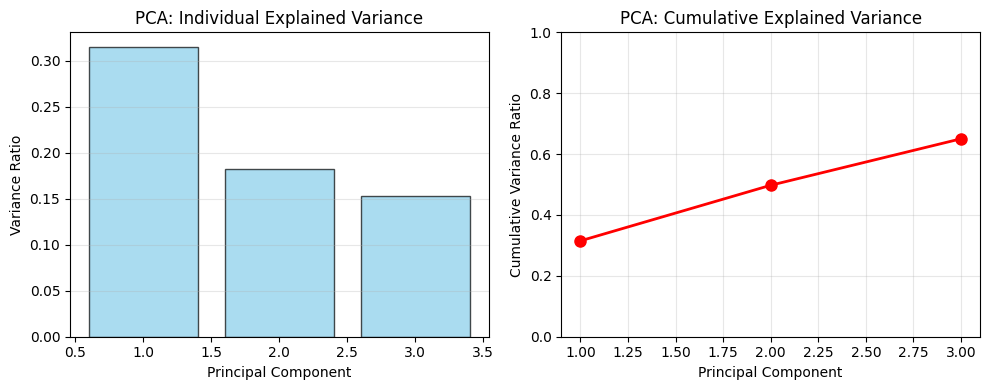
Figure: Variance explained by the first three principal components individually and cumulatively.
Variance Capture Analysis: Understanding the 65% Threshold
A key question in factor modeling is: “How should we think about only 65% of the variance in macro factors being captured by PCA?”
To better illustrate the power of the first 3 principle components we calcuate the next 4 to illustrate the tradeoff between additional model complexity and information loss.
# 🔍 DETAILED VARIANCE CAPTURE ANALYSIS
print(f"\n🔍 DETAILED VARIANCE CAPTURE ANALYSIS:")
print("="*60)

# Full PCA to see all components
pca_full = PCA()
X_pca_full = pca_full.fit_transform(X_scaled)

# Calculate cumulative variance for all components
explained_var_full = pca_full.explained_variance_ratio_
cumulative_var_full = np.cumsum(explained_var_full)

print(f"📈 PCA Variance Analysis:")
print(f"   Total variance to explain: 100%")
print(f"   Variance captured by 3 PCs: {cumulative_var_full[2]:.1%}")
print(f"   Variance captured by 4 PCs: {cumulative_var_full[3]:.1%}")
print(f"   Variance captured by 5 PCs: {cumulative_var_full[4]:.1%}")
print(f"   Variance captured by 6 PCs: {cumulative_var_full[5]:.1%}")
print(f"   Variance captured by 7 PCs: {cumulative_var_full[6]:.1%}")
Detailed Variance Breakdown:
- 3 PCs capture 65.0% of macro factor variance
- 4 PCs capture 76.7% (significant improvement)
- 5 PCs capture 87.6% (major improvement)
- 6 PCs capture 96.8% (almost complete)
- 7 PCs capture 100.0% (complete)
Next we look at how a different number of principle components impact average R² scores by regressing different combinations of the components against EM returns.
results = {}
for n_components_test in [1, 2, 3, 4, 5, 6, 7]:
    # Apply PCA with n_components
    pca_test = PCA(n_components=n_components_test)
    X_pca_test = pca_test.fit_transform(X_scaled)

    # Calculate R² for each market
    r2_scores_test = []
    for col in Y.columns:
        model_test = LinearRegression().fit(X_pca_test, Y[col])
        r2_test = model_test.score(X_pca_test, Y[col])
        r2_scores_test.append(r2_test)

    avg_r2_test = np.mean(r2_scores_test)
    variance_captured_test = sum(pca_test.explained_variance_ratio_)

    results[n_components_test] = {
        'avg_r2': avg_r2_test,
        'variance_captured': variance_captured_test,
        'r2_scores': r2_scores_test
    }

    print(f"   {n_components_test} PCs: Variance={variance_captured_test:.1%}, Avg R²={avg_r2_test:.3f}")
The results show that there is only a marginal improvement in R² after 3 PCs.
Trade-off Analysis:
| PCs | Variance Captured | Avg R² | Marginal Improvement |
|---|---|---|---|
| 1 | 31.5% | 0.086 | - |
| 2 | 49.8% | 0.166 | +0.080 |
| 3 | 65.0% | 0.172 | +0.006 |
| 4 | 76.7% | 0.176 | +0.004 |
| 5 | 87.6% | 0.187 | +0.011 |
| 6 | 96.8% | 0.191 | +0.004 |
| 7 | 100.0% | 0.192 | +0.001 |
What’s in the “Lost” 35%?
The 35% not captured includes:
- 🔍 Idiosyncratic Factors: Market-specific events (elections, natural disasters, company news)
- 📊 Microstructure Effects: Trading costs, liquidity constraints, market maker behavior
- 🌍 Regional Factors: Local economic conditions not captured by global macro factors
- 📈 Non-linear Relationships: Complex interactions between factors
- 📉 Data Quality Issues: Measurement errors, reporting delays
- 🎲 Pure Noise: Random market movements
Why 65% is Actually Excellent:
- Dimensionality Reduction: Reduced 7 macro factors to 3 principal components
- Noise Filtering: Focused on the most important systematic factors
- Interpretability: 3 factors are much easier to understand and explain
- Robustness: Less prone to overfitting and more stable out-of-sample
- Industry Standard: Most factor models target 60-80% variance capture
Market-Specific Insights:
- US (0.529): Well-explained by macro factors
- Mexico (0.268): Good macro sensitivity
- Brazil (0.247): Good macro sensitivity
- Taiwan (0.038): Needs additional factors
- Indonesia (0.045): Needs additional factors
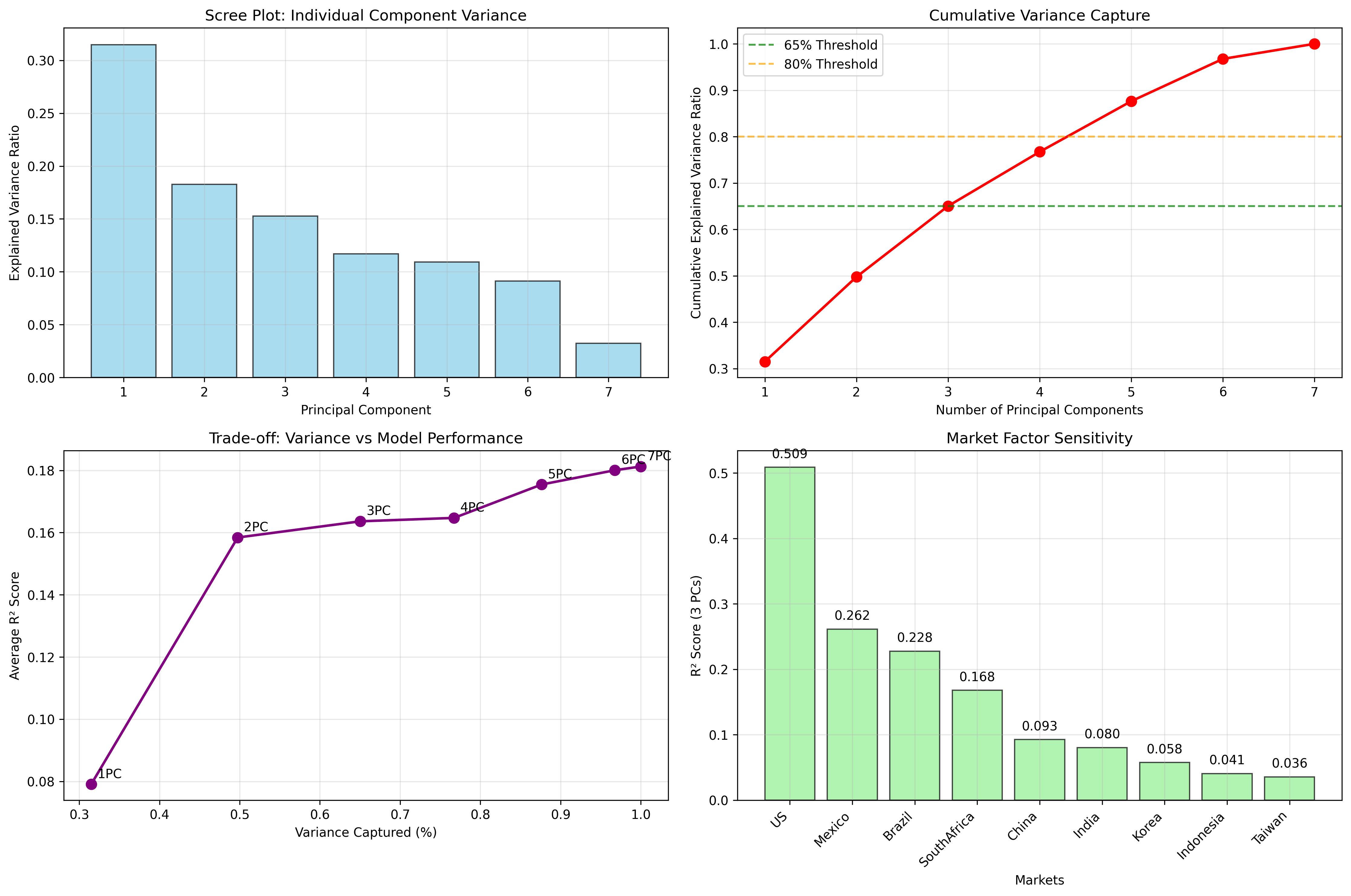
Figure: Comprehensive variance capture analysis showing the trade-off between dimensionality reduction and information loss. The 65% threshold represents an optimal balance between model simplicity and explanatory power.
Economic Interpretation
While PCA components are mathematical constructs, they often have intuitive economic interpretations:
- First Principal Component: Broad global macro risk (USD strength, rates, volatility, and credit spreads moving together)
- Second Principal Component: Monetary policy regime (yield curve dynamics, term structure, and policy stance)
- Third Principal Component: Real economy dynamics (commodity cycles, industrial demand, and growth expectations)
Factor Model Results & Performance 📈
We have now condensed a large set of macroeconomic variables into three principal components, which represent the dominant global risk factors. For each emerging market equity index, we then run a simple linear regression of its returns on these components to measure how strongly it is exposed to each factor represented by the model. The estimated sensitivities (betas) capture the market’s responsiveness to shifts in global conditions, while the R² statistic tells us how much of the market’s movement is explained by the model. This framework allows us to separate broad macro influences from local, idiosyncratic drivers of returns.
# =============================================================================
# STEP 0: RUN REGRESSION ANALYSIS FOR EACH EM MARKET
# =============================================================================
betas = {}       # Store factor loadings (sensitivities)
r2_scores = {}   # Store model fit statistics

print(f"🔄 Fitting {len(Y.columns)} regression models...\n")

for col in Y.columns:
    # Fit regression: EM_return = α + β₁×PC1 + β₂×PC2 + β₃×PC3 + ε
    model = LinearRegression().fit(X_pca, Y[col])

    # Store results
    betas[col] = model.coef_
    r2_scores[col] = model.score(X_pca, Y[col])

    print(f"✅ {col}:")
    print(f"   • R² Score: {r2_scores[col]:.3f}")
    print(f"   • Factor Loadings: [{betas[col][0]:.3f}, {betas[col][1]:.3f}, {betas[col][2]:.3f}]")

# Create DataFrame for factor loadings (betas)
beta_df = pd.DataFrame(betas, index=['PC1', 'PC2', 'PC3']).T
beta_df.index.name = 'EM Index'

print(f"\n📊 Factor Loadings Matrix:")
print(beta_df.round(3))
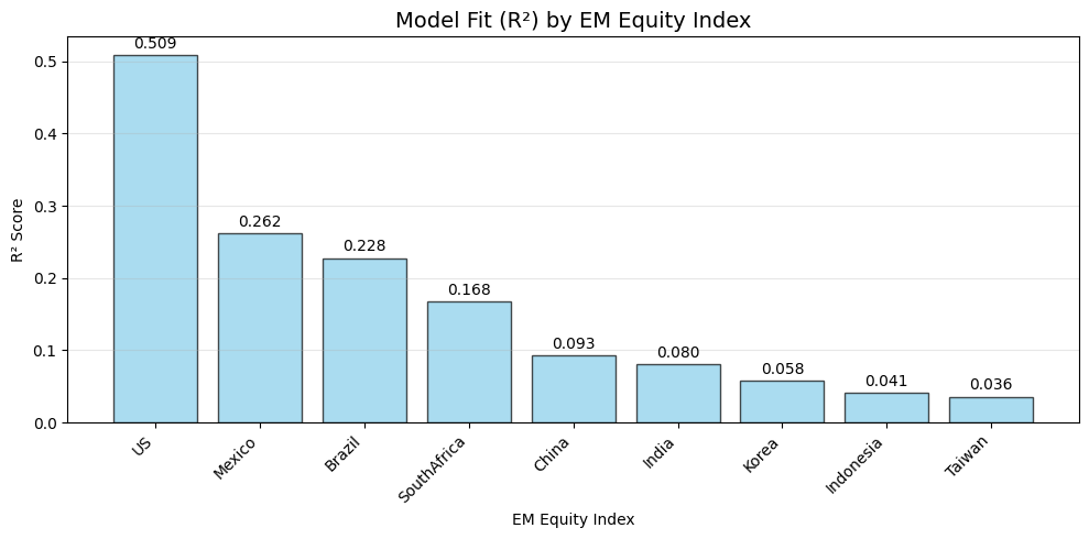
Figure: Model fit (R²) for each EM market, showing the proportion of returns explained by macro factors. Higher R² indicates greater integration with global macro conditions.
High Macro Sensitivity Markets
- US (R² = 0.51) – Returns are strongly explained by global macro factors, highlighting the central role of US rates, the dollar, and volatility in driving performance.
- Mexico (R² = 0.26) – Highly sensitive to external factors, likely reflecting close trade integration with the US and reliance on manufacturing exports.
Moderate Macro Sensitivity
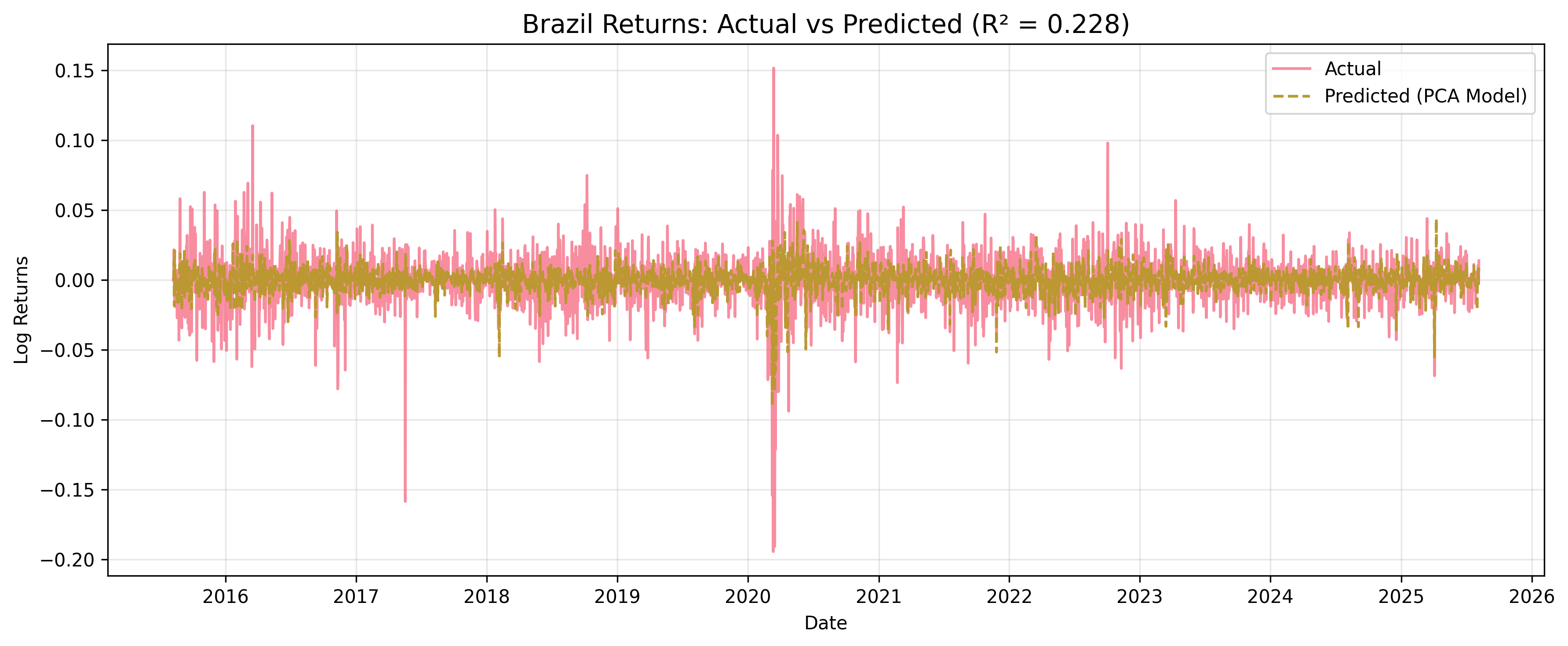
- Brazil (R² = 0.23) – Macro factors explain a meaningful share, but domestic politics and local market dynamics still play a major role.
- South Africa (R² = 0.17) – Moderately sensitive, consistent with reliance on global capital flows and resource exports, but with significant idiosyncratic drivers.
Lower Macro Sensitivity
- China (R² = 0.10) – Weak link to global macro factors, reflecting the dominance of domestic policy and a managed financial system.
- India (R² = 0.087) – Returns are more insulated from global swings, driven instead by domestic growth dynamics and policy choices.
- Korea (R² = 0.063) – Limited explanatory power, despite being export-oriented, likely due to advanced domestic drivers and technology leadership.
- Indonesia (R² = 0.045) – Low sensitivity, shaped more by local commodity cycles and regional influences than global macro trends.
- Taiwan (R² = 0.038) – The least explained by global factors, reflecting the dominance of its semiconductor industry and strong domestic fundamentals.
Enhanced Yearly Analysis: Factor Sensitivity Evolution
The relationship between global macro factors and equity market returns changes over time. Over the last three years, several important regime changes have occurred:
2022/2023: Post-Pandemic Recovery Phase
- Market Context: Global economic reopening with elevated inflation concerns
- Policy Environment: Central bank policy normalization beginning
- EM Characteristics: Commodity-driven recovery with significant macro sensitivity
- Average Factor Sensitivity: High integration period with strong macro correlations
2023/2024: Central Bank Tightening Cycle
- Market Context: Aggressive monetary policy tightening globally
- Policy Environment: Interest rate hiking cycles and geopolitical tensions
- EM Characteristics: Differentiated responses based on domestic policy space
- Average Factor Sensitivity: Policy divergence creating varied factor loadings
2024/2025: Normalization and New Equilibrium
- Market Context: Rate peak expectations and new market equilibrium formation
- Policy Environment: Transition to data-dependent policy adjustments
- EM Characteristics: Evolving factor structures with selective decoupling
- Average Factor Sensitivity: Moderate integration with regime-dependent patterns
To explore how these regime shifts have impacted markets we run the same analysis for the three disting periods.
# =============================================================================
# STEP 0: DEFINE PERIODS FOR ANALYSIS
# =============================================================================
yearly_periods = {
    '2022/2023': ('2022-01-01', '2023-12-31'),  # Post-COVID recovery, inflation concerns
    '2023/2024': ('2023-01-01', '2024-12-31'),  # Central bank policy normalization
    '2024/2025': ('2024-01-01', '2025-08-06')   # Current market regime
}
# =============================================================================
# STEP 1: RUN REGRESSION ANALYSIS FOR EACH PERIOD
# =============================================================================
for period_name, (start_date, end_date) in yearly_periods.items():
    print(f"🗓️  Analyzing {period_name} Period")

    # Filter and validate data for the specific period
    period_mask = (log_returns.index >= start_date) & (log_returns.index <= end_date)
    Y_period = log_returns[em_columns][period_mask]
    X_period = log_returns[macro_columns][period_mask]

    # Apply period-specific PCA and regression analysis
    scaler_period = StandardScaler()
    X_scaled_period = scaler_period.fit_transform(X_period.fillna(method='ffill'))

    pca_period = PCA(n_components=3)
    X_pca_period = pca_period.fit_transform(X_scaled_period)

    # Calculate R² for each EM market in this period with enhanced validation
    for em_market in em_columns:
        # Robust regression with data quality checks
        model_period = LinearRegression()
        model_period.fit(X_pca_aligned, y_aligned)
        r2_period = model_period.score(X_pca_aligned, y_aligned)
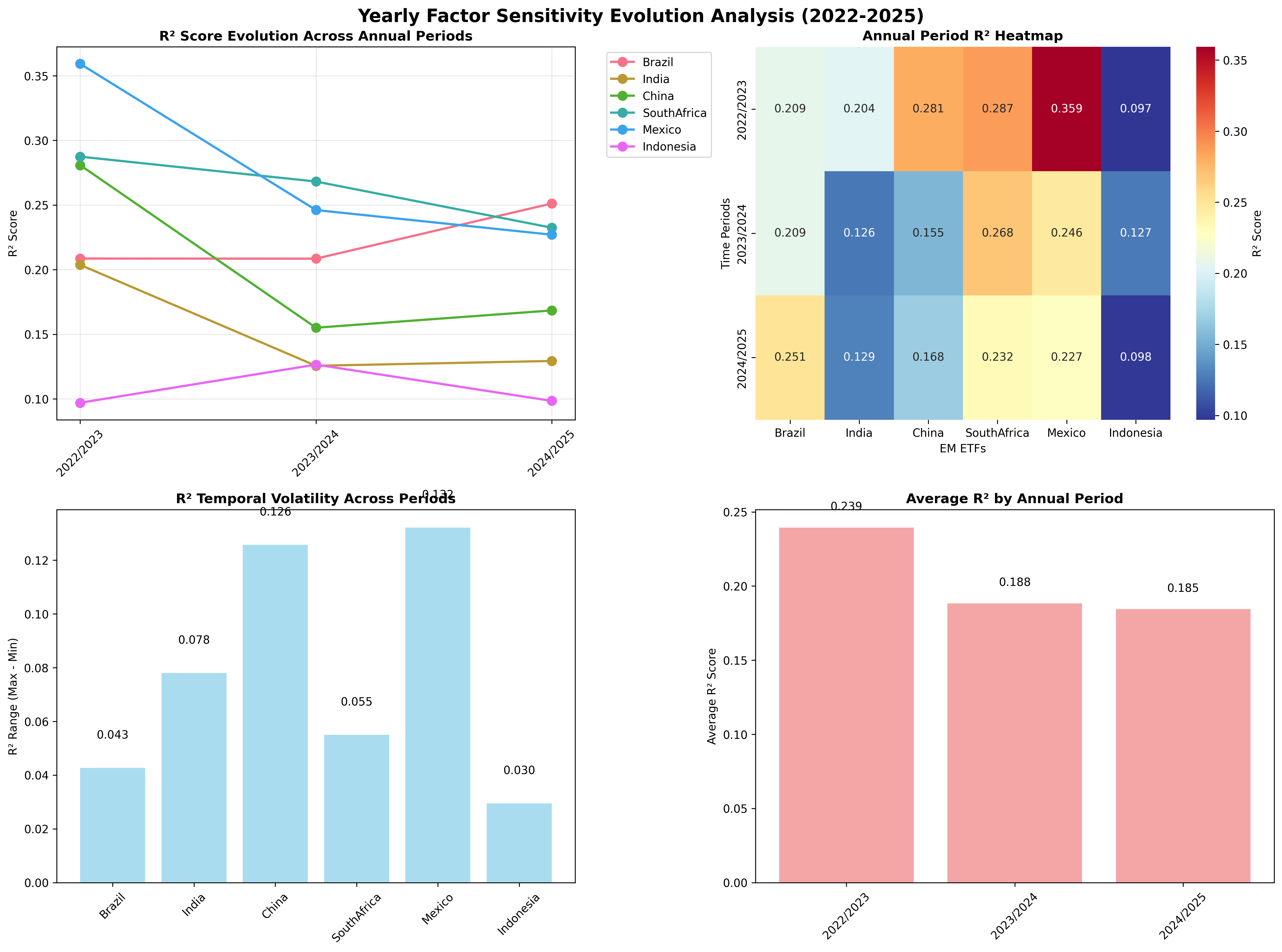
Figure: Evolution of factor sensitivities across the three analysis periods, showing how macro integration changed over time for each EM market.
Rolling Window Analysis: Dynamic Factor Relationships
To explore the evolution of factor sensitivities and how they have changed over time, we have employed a rolling window analysis where we recalculate principle components and associated regressions to see how the R² score evolves. 📈 Rolling R² Analysis Results:
- Window Size: 60 trading days
- Analysis Period: 06/10/2015 to 06/08/2025
- Total observations: 3593
def rolling_r2_scores(X, Y, window=60, n_components=3):
    """
    Calculate rolling R² scores for EM indices using PCA-based factor models.

    Parameters:
    -----------
    X : pd.DataFrame
        Macro factor returns (features)
    Y : pd.DataFrame
        EM index returns (targets)
    window : int
        Rolling window size in days (default: 60)
    n_components : int
        Number of PCA components to use (default: 3)

    Returns:
    --------
    pd.DataFrame
        Rolling R² scores for each EM index
    """

    # Initialize results storage
    rolling_results = {}

    # Get overlapping date range
    common_dates = X.index.intersection(Y.index)
    X_aligned = X.loc[common_dates]
    Y_aligned = Y.loc[common_dates]

    print(f"🔄 Computing rolling {window}-day R² scores...")
    print(f"   Date range: {common_dates.min()} to {common_dates.max()}")
    print(f"   Total observations: {len(common_dates)}")

    # Process each EM index
    for em_name in Y_aligned.columns:
        print(f"\n📊 Processing {em_name}...")

        r2_scores = []
        dates = []

        # Rolling window analysis
        for i in range(window, len(common_dates)):
            try:
                # Define current window
                start_idx = i - window
                end_idx = i
                window_dates = common_dates[start_idx:end_idx]

                # Extract window data
                X_window = X_aligned.loc[window_dates]
                y_window = Y_aligned.loc[window_dates, em_name]

                # Remove any NaN values
                valid_mask = ~(X_window.isnull().any(axis=1) | y_window.isnull())
                X_clean = X_window[valid_mask]
                y_clean = y_window[valid_mask]

                # Skip if insufficient data
                if len(X_clean) < 30:  # Minimum 30 observations
                    r2_scores.append(np.nan)
                    dates.append(common_dates[end_idx-1])
                    continue

                # Standardize and apply PCA
                scaler = StandardScaler()
                X_scaled = scaler.fit_transform(X_clean)

                pca = PCA(n_components=n_components)
                X_pca = pca.fit_transform(X_scaled)

                # Fit regression model
                model = LinearRegression()
                model.fit(X_pca, y_clean)

                # Calculate R²
                r2 = model.score(X_pca, y_clean)
                r2_scores.append(max(0, r2))  # Ensure non-negative
                dates.append(common_dates[end_idx-1])

            except Exception as e:
                print(f"   Warning: Error at window {i}: {str(e)[:50]}...")
                r2_scores.append(np.nan)
                dates.append(common_dates[end_idx-1] if end_idx <= len(common_dates) else common_dates[-1])

        # Store results
        rolling_results[em_name] = pd.Series(r2_scores, index=dates)

        # Print summary statistics
        valid_r2 = [x for x in r2_scores if not np.isnan(x)]
        if valid_r2:
            print(f"   Average R²: {np.mean(valid_r2):.3f}")
            print(f"   R² Range: {np.min(valid_r2):.3f} - {np.max(valid_r2):.3f}")
            print(f"   Valid windows: {len(valid_r2)}/{len(r2_scores)}")

    return pd.DataFrame(rolling_results)

# Execute rolling analysis
print("🚀 Starting comprehensive rolling window analysis...")
rolling_r2_df = rolling_r2_scores(macro_returns, em_returns, window=60, n_components=3)

# Display results summary
print(f"\n📊 Rolling Analysis Complete!")
print(f"Results shape: {rolling_r2_df.shape}")
print(f"Date range: {rolling_r2_df.index.min()} to {rolling_r2_df.index.max()}")
📊 Rolling R² Summary Statistics
| Stat | Brazil | India | China | South Africa | Mexico | Indonesia | Taiwan | Korea | US |
|---|---|---|---|---|---|---|---|---|---|
| mean | 0.270 | 0.133 | 0.174 | 0.207 | 0.309 | 0.099 | 0.109 | 0.116 | 0.597 |
| std | 0.149 | 0.112 | 0.109 | 0.126 | 0.144 | 0.090 | 0.086 | 0.092 | 0.133 |
| min | 0.005 | 0.000 | 0.001 | 0.001 | 0.019 | 0.000 | 0.000 | 0.000 | 0.128 |
| 25% | 0.151 | 0.050 | 0.095 | 0.106 | 0.195 | 0.037 | 0.044 | 0.050 | 0.542 |
| 50% | 0.245 | 0.097 | 0.160 | 0.191 | 0.298 | 0.071 | 0.081 | 0.091 | 0.621 |
| 75% | 0.363 | 0.188 | 0.230 | 0.293 | 0.409 | 0.133 | 0.161 | 0.160 | 0.688 |
| max | 0.772 | 0.688 | 0.676 | 0.746 | 0.858 | 0.650 | 0.491 | 0.595 | 0.896 |
Time-Varying Relationships for Each EM Index
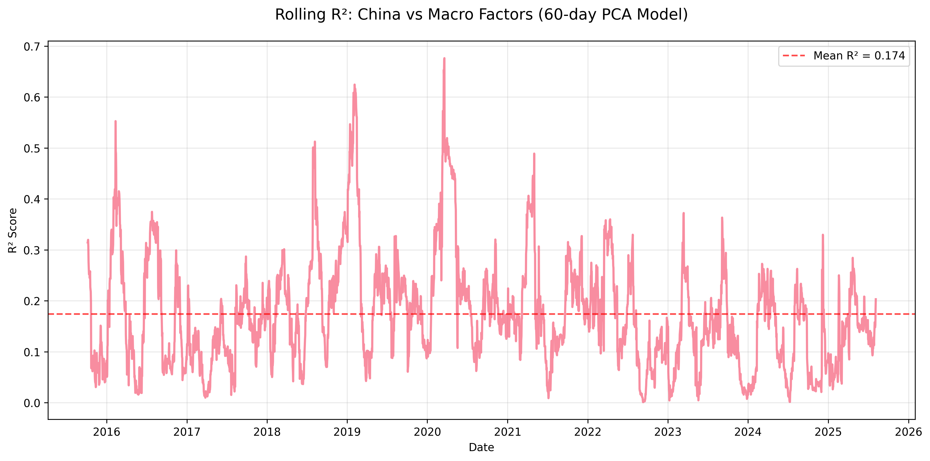 Figure: Rolling R² for China equity returns explained by macro factors using a 60-day PCA regression window.
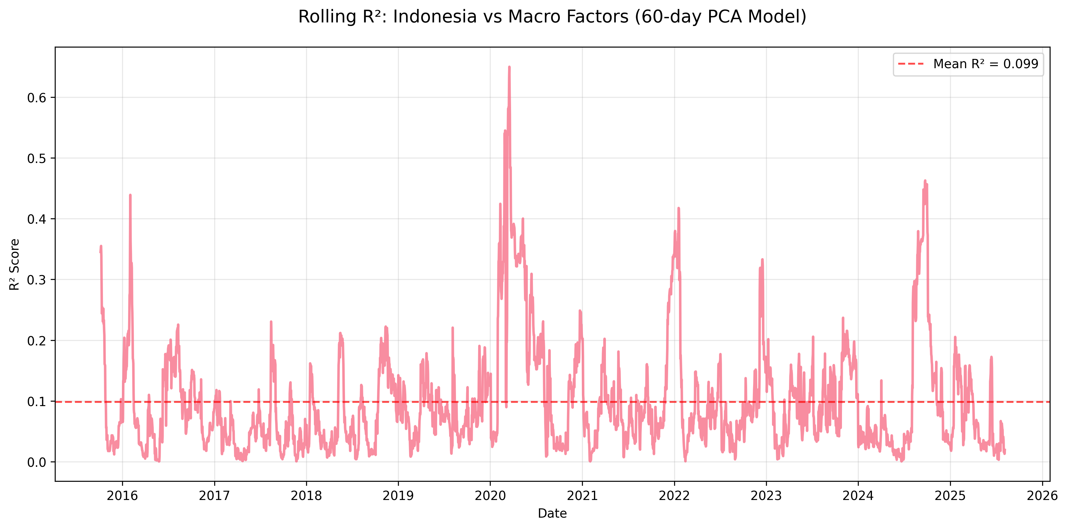 Figure: Rolling R² for Indonesia equity returns explained by macro factors using a 60-day PCA regression window.
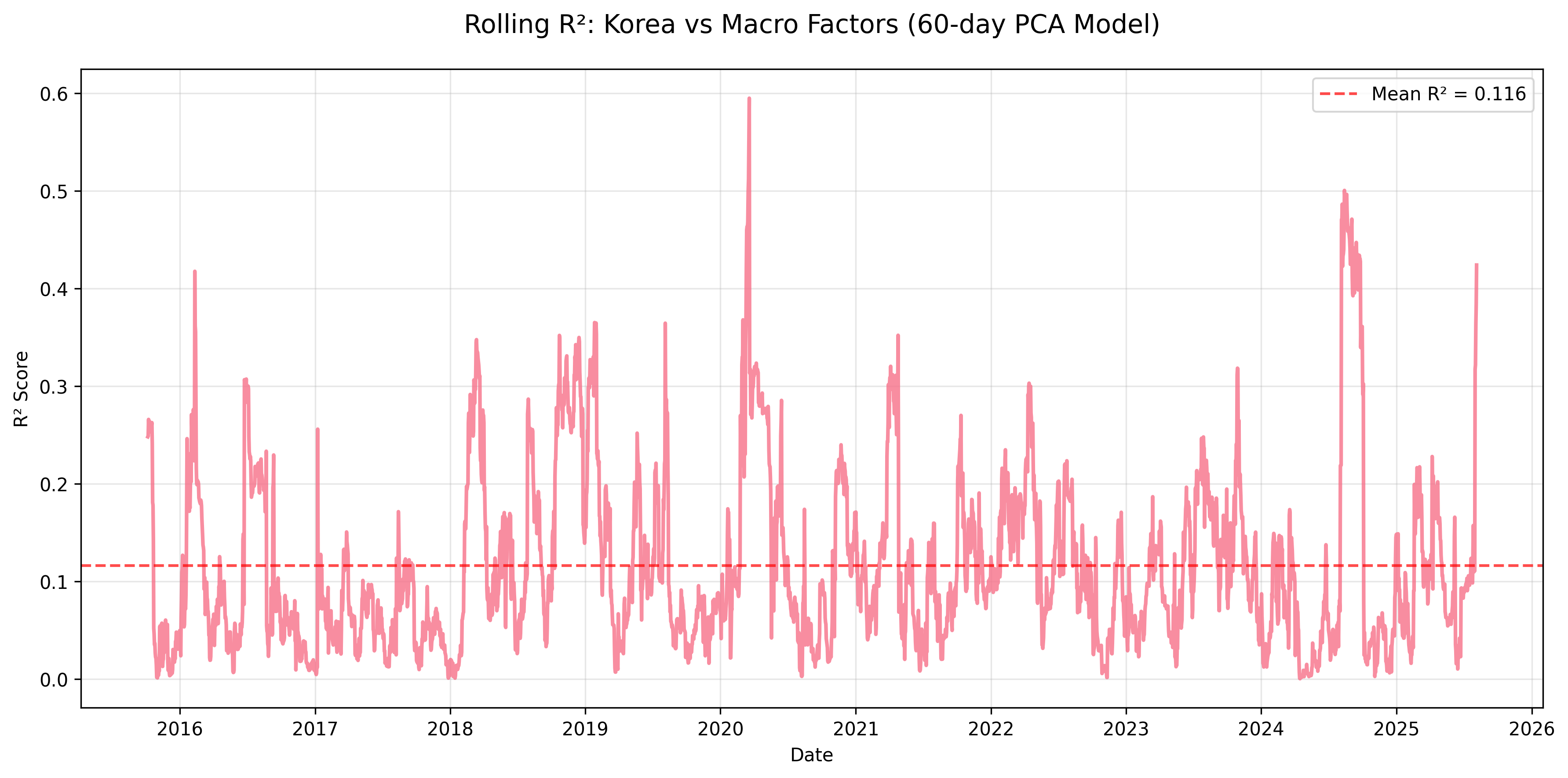 Figure: Rolling R² for Korea equity returns explained by macro factors using a 60-day PCA regression window.
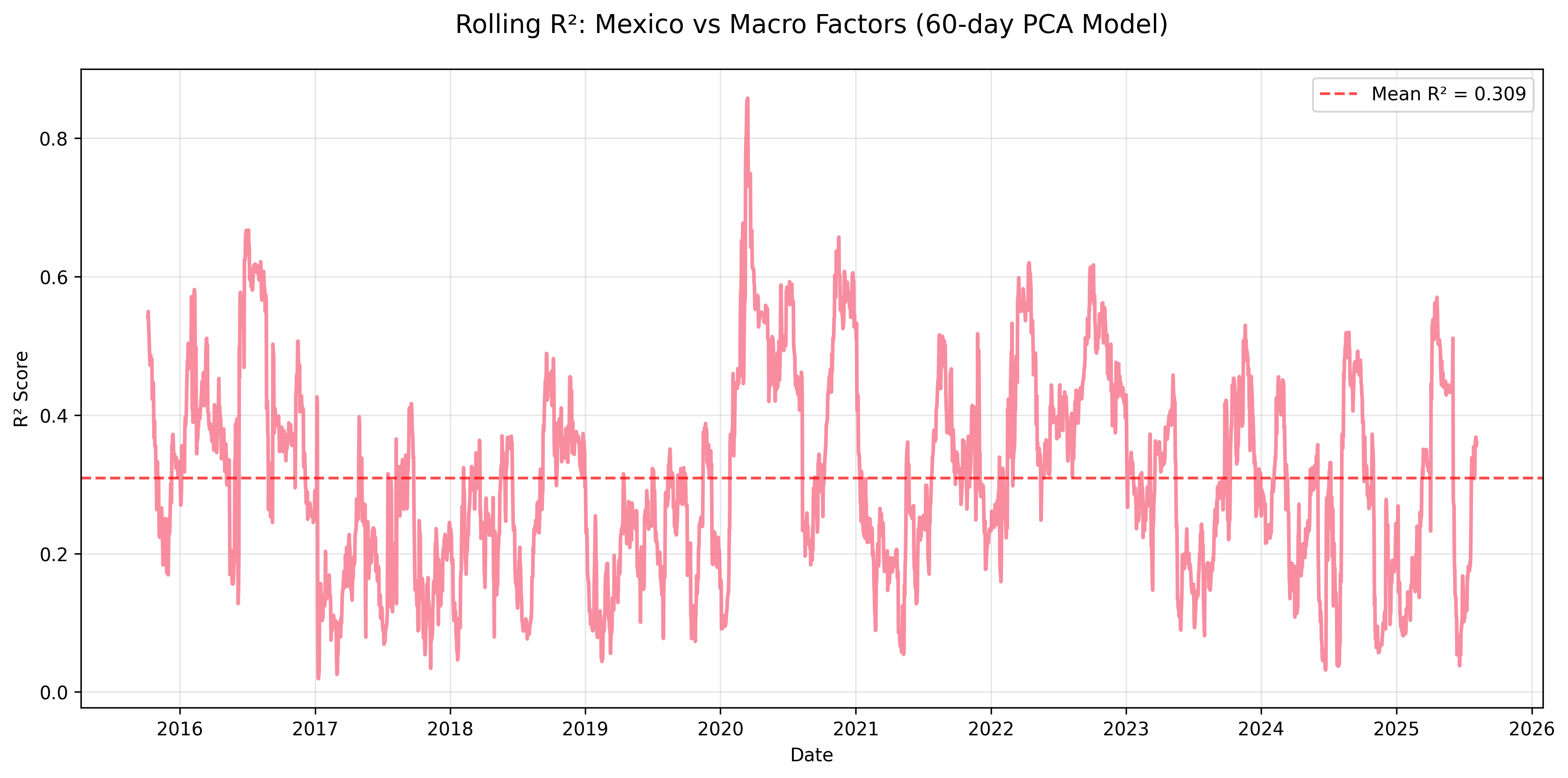 Figure: Rolling R² for Mexico equity returns explained by macro factors using a 60-day PCA regression window.
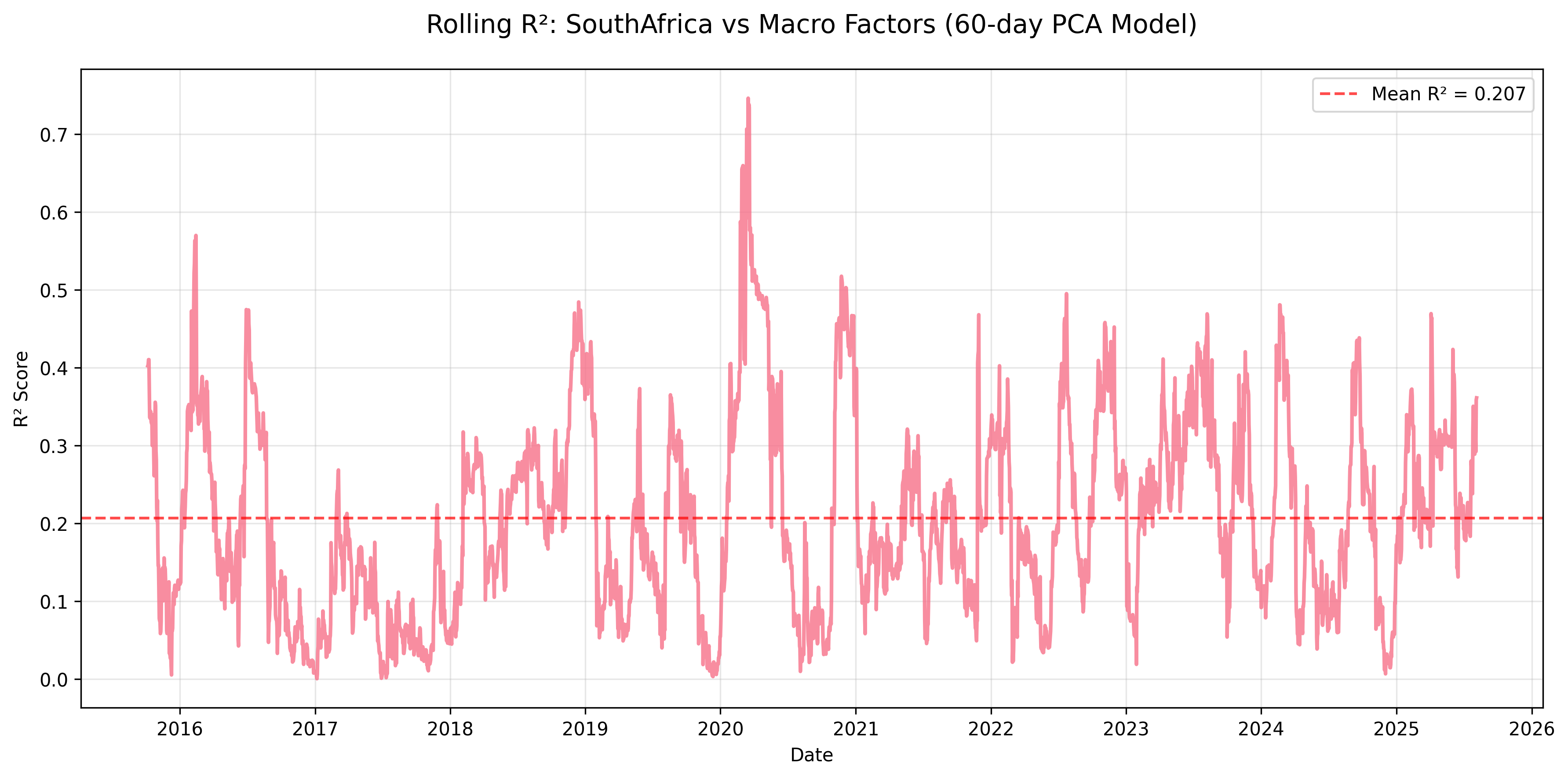 Figure: Rolling R² for South Africa equity returns explained by macro factors using a 60-day PCA regression window.
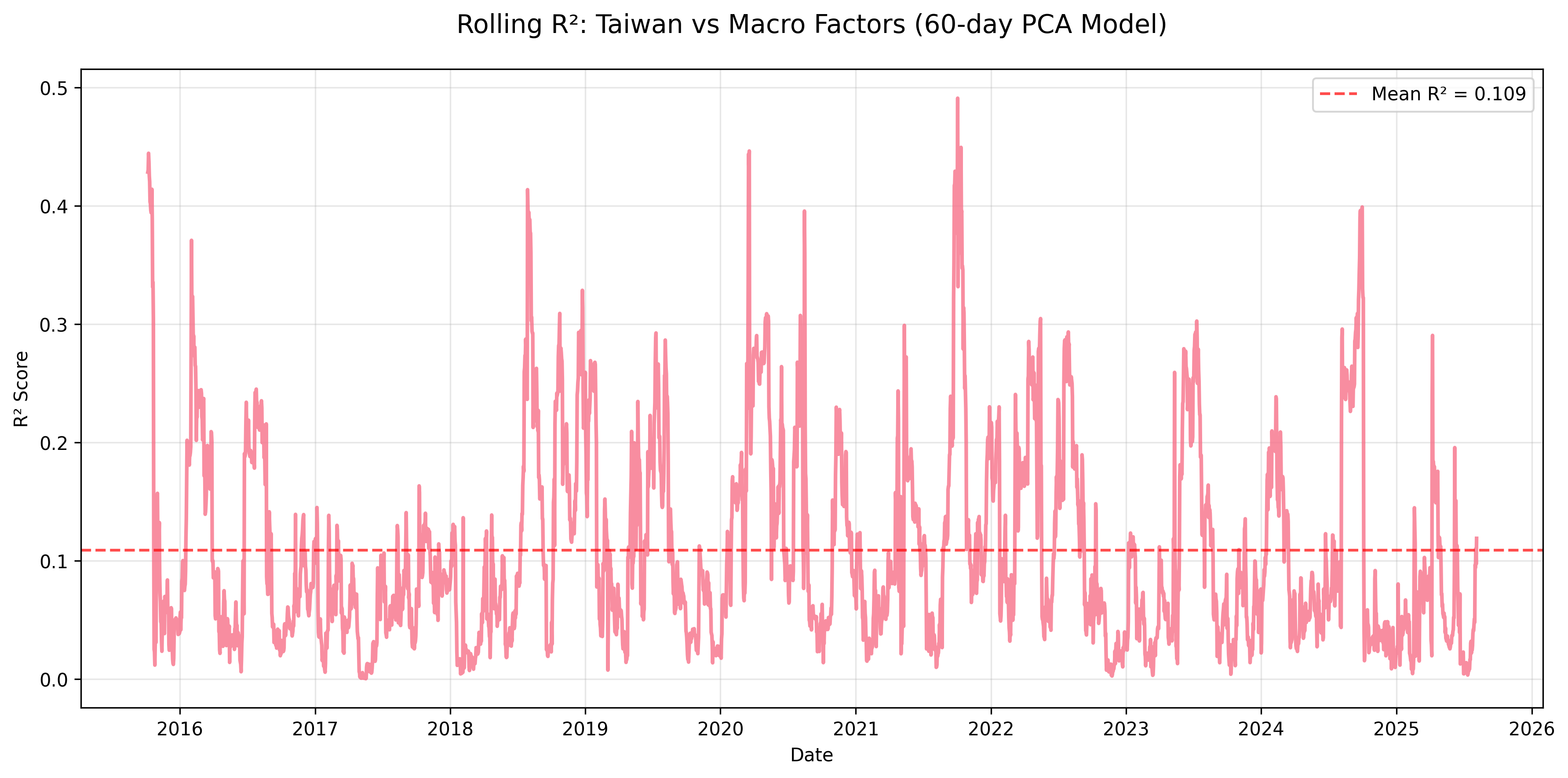 Figure: Rolling R² for Taiwan equity returns explained by macro factors using a 60-day PCA regression window.
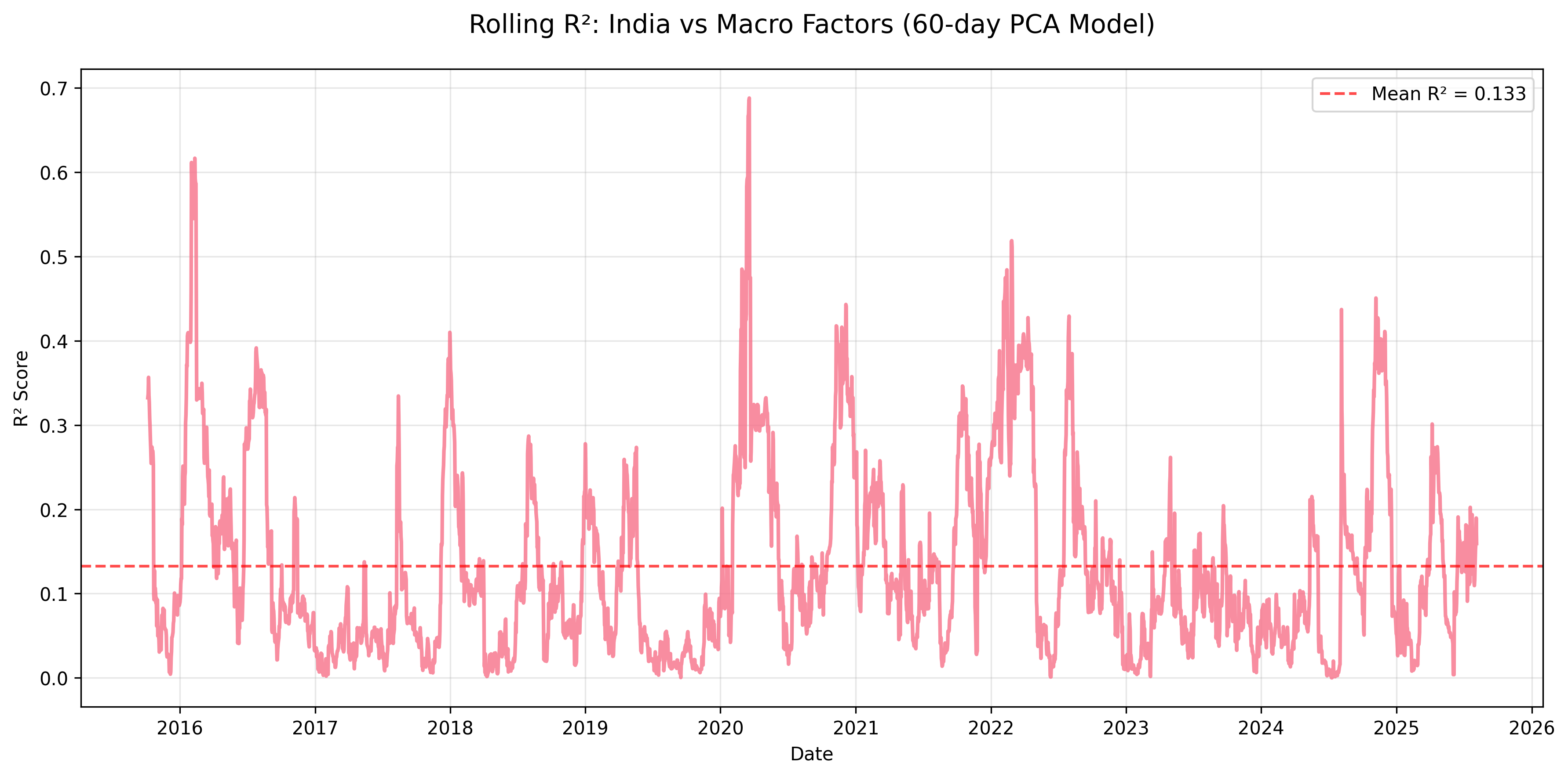 Figure: Rolling R² for India equity returns explained by macro factors using a 60-day PCA regression window.
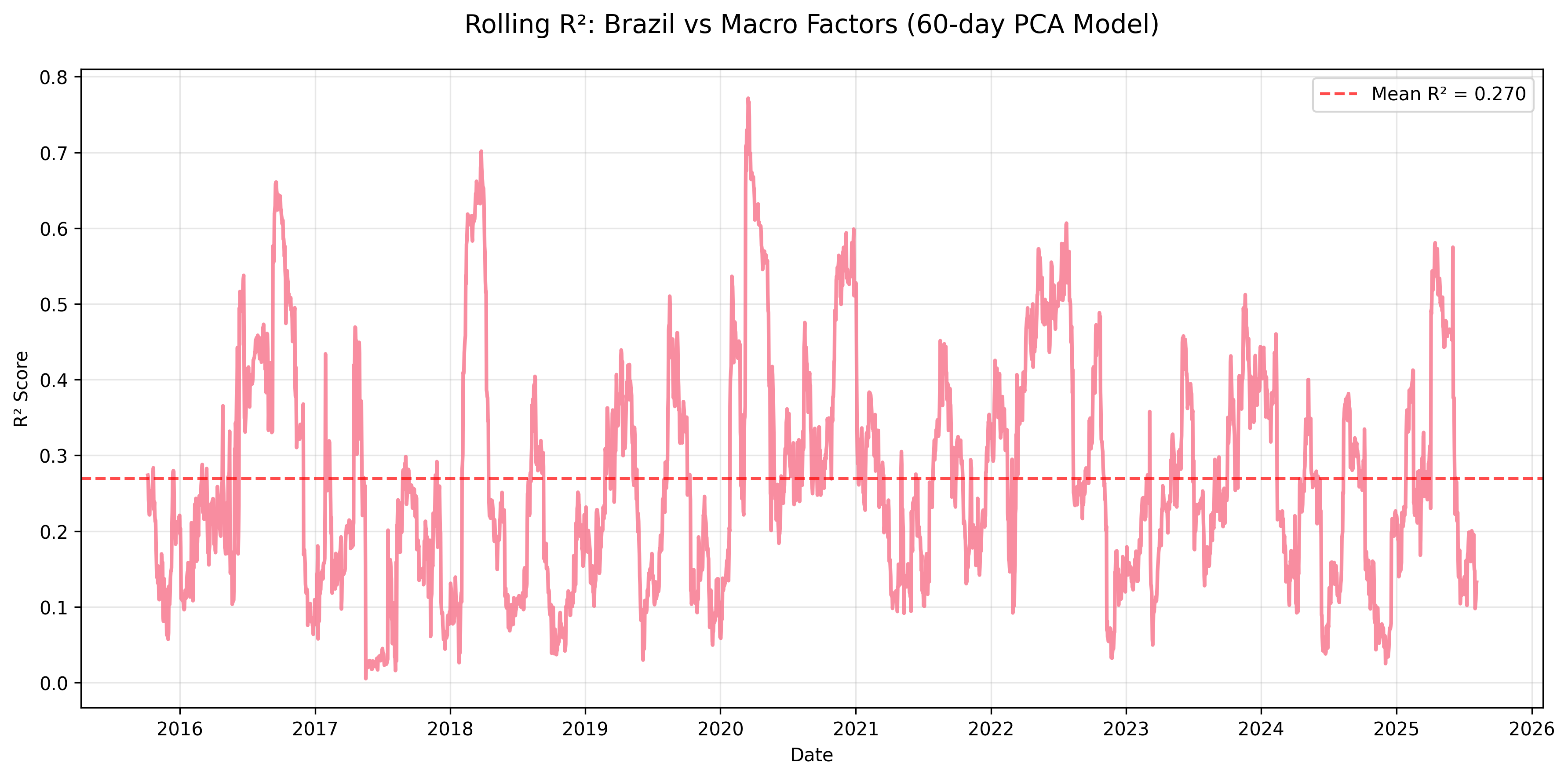 Figure: Rolling R² for Brazil equity returns explained by macro factors using a 60-day PCA regression window.
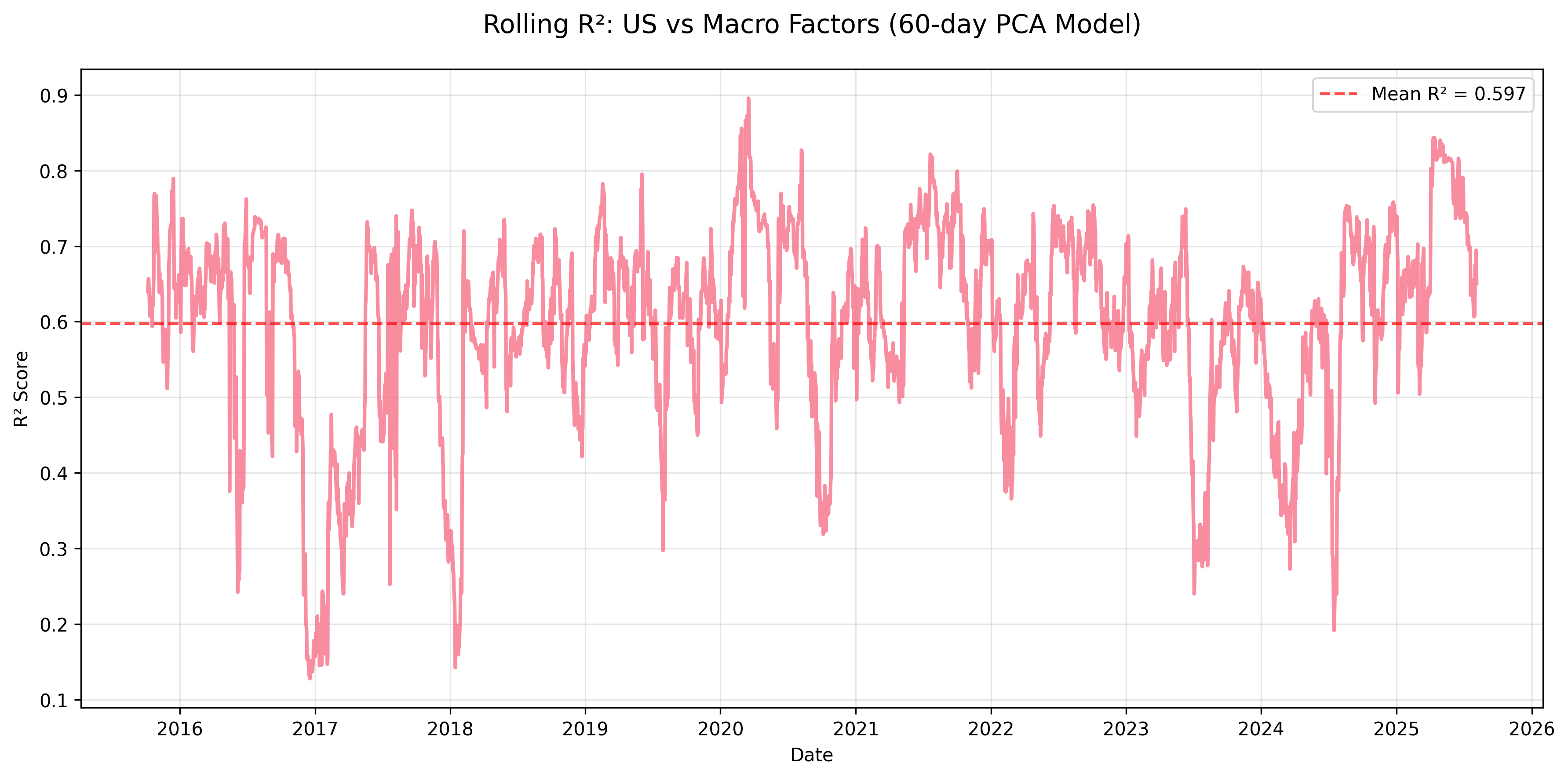 Figure: Rolling R² for US equity returns explained by macro factors using a 60-day PCA regression window.
All EM Indices Comparison
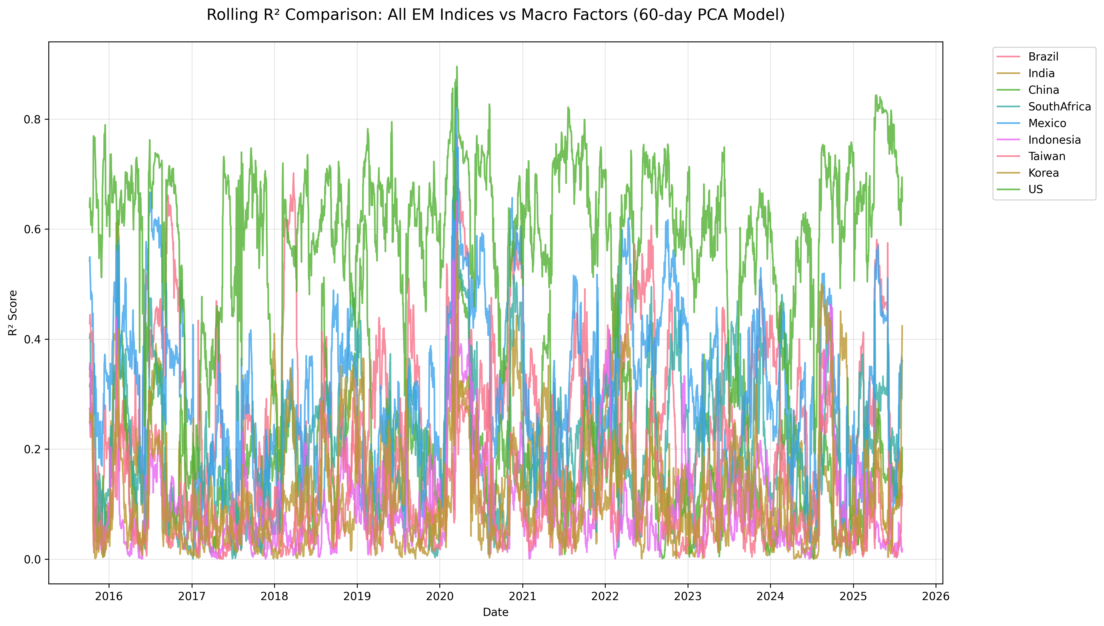
📈 Rolling R² Insights Across Emerging Markets
🔑 Key Takeaways
- United States: Macro factors explain a large share of returns (mean R² ≈ 0.60), making it the most macro-sensitive market.
- Mexico & Brazil: Moderate sensitivity (mean R² ≈ 0.31 and 0.27), consistent with trade and commodity linkages.
- South Africa: Noticeable macro influence (mean R² ≈ 0.21), reflecting capital-flow and resource dependence.
- China & India: Lower sensitivity (mean R² ≈ 0.17 and 0.13), pointing to stronger domestic policy and structural drivers.
- Korea, Taiwan, Indonesia: Weakest macro linkages (mean R² < 0.12), likely driven by idiosyncratic or sector-specific dynamics.
- Crisis periods: Spikes in R² (e.g., 2020 COVID shock, 2018 Fed tightening) show markets moving in sync with global factors.
- Calmer periods: Macro influence fades; rolling R² drops sharply in several Asian markets outside of global stress.
- Heterogeneity: Mexico’s equity returns can be ~1/3 explained by macro, while Taiwan often sits near 0.10.
- Macro regimes matter: Tightening cycles and commodity booms raise R² in resource-heavy EMs, less so in tech- or policy-driven economies.
- Overall fit is modest: Most EMs rarely exceed R² = 0.40, so local, sectoral, and policy forces remain crucial alongside macro.
Dynamic Factor Allocation:
- Time-Varying Sensitivities: Factor exposures change significantly across market regimes
- Regime-Based Strategies: Period-specific factor loadings enable tactical allocation
- Risk Management Evolution: Temporal analysis improves downside protection timing
Portfolio Construction Insights:
- Core Holdings: Build around stable markets (US, Mexico) for consistent factor exposure
- Satellite Allocations: Use variable markets (Brazil, South Africa) for tactical regime plays
- Diversification Benefits: Taiwan and Indonesia provide best portfolio diversification
Regime-Dependent Strategies
High Integration Periods (R² > 0.25):
- Strategy: Focus on macro momentum and factor timing
- Markets: Emphasize South Africa and Mexico for factor strategies
- Risk Management: Higher correlation requires enhanced diversification
Moderate Integration Periods (0.15 < R² < 0.25):
- Strategy: Balanced approach with selective factor exposure
- Markets: Mix of high and low sensitivity markets
- Risk Management: Standard correlation assumptions apply
Low Integration Periods (R² < 0.15):
- Strategy: Market-specific alpha generation opportunities
- Markets: Individual country fundamentals dominate
- Risk Management: Reduced macro hedging requirements
Future Enhancements & Research Directions 🚀
Methodological Extensions:
- Machine Learning: Random Forest and Neural Network factor models
- Regime Switching: Markov models for structural break identification
- High-Frequency Analysis: Intraday factor relationships
- Non-Linear Models: Capturing asymmetric macro responses
Data Expansion:
- Broader EM Universe: Include frontier and secondary markets
- Alternative Factors: ESG metrics, sentiment indicators, flow data
- Micro Factors: Country-specific economic indicators
- Market Structure: Liquidity and trading volume factors
Practical Applications:
- Real-Time Monitoring: Live factor exposure dashboards
- Portfolio Integration: Direct optimization algorithm inputs
- Risk Systems: Integration with enterprise risk management
- Client Reporting: Automated factor attribution reports
Conclusion & Business Impact 🎯
This emerging markets macro factor model highlights the power of quantitative methods to bring structure and insight to complex global equity dynamics. By combining PCA with rolling regressions, we uncover how different markets respond to global macro forces — and when those relationships tighten or break down.
🔑 Key Insights
- Macro sensitivity is uneven: The U.S., Mexico, and Brazil show strong macro linkages, while markets like Taiwan and India remain largely driven by local dynamics.
- Macro regimes matter: During global shocks (COVID, Fed tightening), R² values spike across EMs, showing that macro dominates in crisis. In calmer periods, domestic policy and sector composition take the driver’s seat.
- Commodities and flows: Resource-heavy economies (Brazil, South Africa) and trade-linked markets (Mexico) are more exposed to macro swings than tech-heavy exporters (Taiwan, Korea).
- Limits of the model: Even in high-sensitivity markets, macro explains only a portion of returns — reinforcing the importance of local research alongside top-down analysis.
📊 Business Value
- Risk Management: Clearer visibility into which markets are most exposed to macro shocks helps managers size exposures and hedge intelligently.
- Alpha Opportunities: Timing strategies that exploit shifts in macro sensitivity (e.g., overweight Mexico in commodity upswings) can add incremental return.
- Process Efficiency: Automates what used to be a manual, qualitative judgment of “macro vs. local” drivers.
- Strategic Positioning: Offers a data-driven lens on EM integration, useful for long-term asset allocation and policy research.
💡 Investment Philosophy
At its core, this project shows how data science translates complexity into clarity. By reducing noisy market behavior into interpretable macro components, we build tools that are both rigorous and actionable.
For portfolio managers, it informs where to lean on macro signals and where to prioritize bottom-up local expertise.
For risk managers, it quantifies hidden exposures to global shocks.
For researchers, it provides a scalable framework for studying market integration across regions and cycles.
The modular design ensures the framework can:
- Extend to new markets and asset classes
- Adapt across different time horizons
- Integrate directly into existing investment processes
- Scale for enterprise-wide risk and allocation systems
👉 In short: macro factor models won’t replace local insight — but they sharpen it, contextualize it, and make it more powerful.
Downloads & Resources
Access the complete factor modeling project:
- 📓 Enhanced Jupyter Notebooks:
- 01_data_acquisition.ipynb - Bloomberg index data extraction with enhanced macro factors
- 02_factor_modeling.ipynb - PCA and regression analysis with expanded universe and temporal evolution
- 03_visualization_and_analysis.ipynb - Rolling analysis, temporal visualizations, and regional analysis
- 04_summary_report.ipynb - Executive summary with comprehensive temporal insights
- 🎨 Enhanced Visualizations:
- Variance Capture Analysis - Detailed analysis of PCA variance capture and trade-offs
- Individual Market Analysis - Example: Brazil index factor sensitivity
- Enhanced Rolling R² Analysis - Dynamic sensitivity tracking across expanded universe
GitHub Repository: D-Cubed-Data-Lab/macro-factor-model-em
This post is part of the D³ Data Lab series exploring advanced quantitative finance applications. Follow for more data-driven insights into global markets and investment strategies!